Seaborn을 활용한 다양한 그래프 그리기
- 0. Seaborn 개요
- 1. Scatterplot
- 2. Barplot, Barhplot
- 3. Line Plot
- 4. Areaplot (Filled Area)
- 5.Histogram
- 6. Pie Chart
- 7. Box Plot
reference:
1 | import numpy as np |
1 | plt.rcParams["figure.figsize"] = (9, 6) # figure size 설정 |
0. Seaborn 개요
seaborn은 matplotlib을 더 사용하게 쉽게 해주는 라이브러리다.
matplotlib으로 대부분의 시각화는 가능하지만, 다음과 같은 이유로 많은 사람들이 seaborn을 선호한다.
0-1. seaborn 에서만 제공되는 통계 기반 plot
1 | tips = sns.load_dataset("tips") |
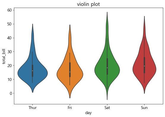
(1) violinplot
1 | sns.violinplot(x="day", y="total_bill", data=tips) |
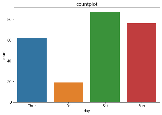
(2) countplot
1 | sns.countplot(tips['day']) |
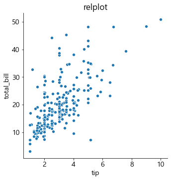
(3) relplot
1 | sns.relplot(x='tip', y='total_bill', data=tips) |
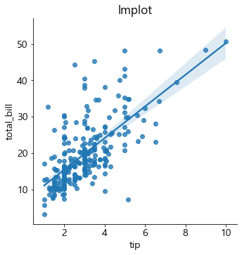
(4) lmplot
1 | sns.lmplot(x='tip', y='total_bill', data=tips) |
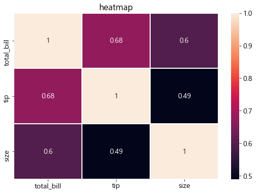
(5) heatmap
1 | plt.title('heatmap') |
0-2. 아름다운 스타일링
(1) default color의 예쁜 조합
seaborn의 최대 장점 중의 하나가 아름다운 컬러팔레트다.
스타일링에 크게 신경 쓰지 않아도 default 컬러가 예쁘게 조합해준다.
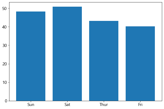
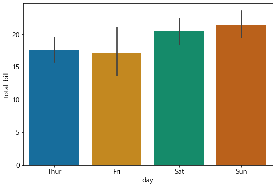
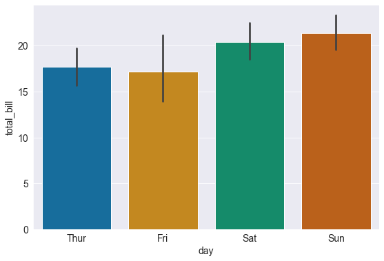
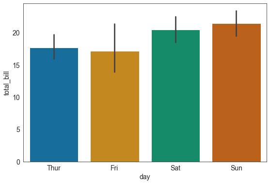
matplotlib VS seaborn
1 | plt.bar(tips['day'], tips['total_bill']) |
1 | sns.barplot(x="day", y="total_bill", data=tips, palette="colorblind") |
(2) 그래프 배경 설정
그래프의 배경 (grid 스타일)을 설정할 수 있음.
sns.set_style(’…’)
- whitegrid: white background + grid
- darkgrid: dark background + grid
- white: white background (without grid)
- dark: dark background (without grid)
1 | sns.set_style('darkgrid') |
1 | sns.set_style('white') |
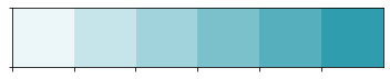
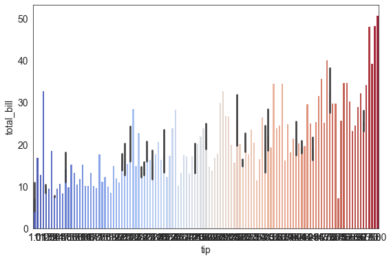
0-3. 컬러 팔레트
자세한 컬러팔레트는 공식 도큐먼트를 참고
1 | sns.palplot(sns.light_palette((210, 90, 60), input="husl")) |


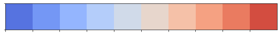

1 | sns.barplot(x="tip", y="total_bill", data=tips, palette='coolwarm') |
<matplotlib.axes._subplots.AxesSubplot at 0x1ba5bf62888>
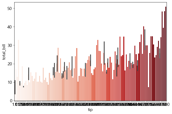
1 | sns.barplot(x="tip", y="total_bill", data=tips, palette='Reds') |
<matplotlib.axes._subplots.AxesSubplot at 0x1ba59e40988>
0-4. pandas 데이터프레임과 높은 호환성
1 | tips |
| total_bill | tip | sex | smoker | day | time | size | |
|---|---|---|---|---|---|---|---|
| 0 | 16.99 | 1.01 | Female | No | Sun | Dinner | 2 |
| 1 | 10.34 | 1.66 | Male | No | Sun | Dinner | 3 |
| 2 | 21.01 | 3.50 | Male | No | Sun | Dinner | 3 |
| 3 | 23.68 | 3.31 | Male | No | Sun | Dinner | 2 |
| 4 | 24.59 | 3.61 | Female | No | Sun | Dinner | 4 |
| ... | ... | ... | ... | ... | ... | ... | ... |
| 239 | 29.03 | 5.92 | Male | No | Sat | Dinner | 3 |
| 240 | 27.18 | 2.00 | Female | Yes | Sat | Dinner | 2 |
| 241 | 22.67 | 2.00 | Male | Yes | Sat | Dinner | 2 |
| 242 | 17.82 | 1.75 | Male | No | Sat | Dinner | 2 |
| 243 | 18.78 | 3.00 | Female | No | Thur | Dinner | 2 |
244 rows × 7 columns
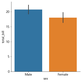
1 | sns.catplot(x="sex", y="total_bill", |
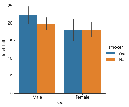
hue옵션: bar를 새로운 기준으로 분할
1 | sns.catplot(x="sex", y="total_bill", |
col/row옵션: 그래프 자체를 새로운 기준으로 분할
1 | sns.catplot(x="sex", y="total_bill", |
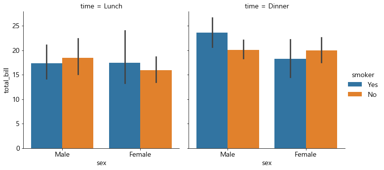
-
xtick, ytick, xlabel, ylabel을 알아서 생성해 줌
-
legend까지 자동으로 생성해 줌
-
뿐만 아니라, 신뢰 구간도 알아서 계산하여 생성함
1. Scatterplot
reference: <sns.scatterplot> Document
sns.scatterplot ( x, y, size=None, sizes=None, hue=None, palette=None, color=‘auto’, alpha=‘auto’… )
sizes옵션: size의 선택범위를 설정. (사아즈의 min, max를 설정)hue옵션: 컬러의 구별 기준이 되는 grouping variable 설정color옵션: cmap에 컬러를 지정하면, 컬러 값을 모두 같게 가겨갈 수 있음alpha옵션: 투명도 (0~1)
1 | sns.set_style('darkgrid') |
1-1. x, y, color, area 설정하기
1 | # 데이터 생성 |
(1) matplotlib
1 | plt.scatter(x, y, s=area, c=colors) |
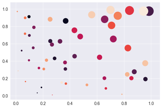
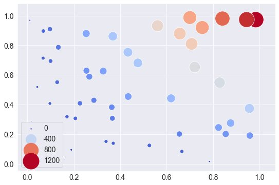
(2) seaborn
1 | sns.scatterplot(x, y, size=area, sizes=(area.min(), area.max()), hue=area, palette='coolwarm') |
[Tip] Palette 이름이 생각안나면: palette 값을 임의로 주고 실행하여 오류 경고창에 정확한 palette 이름을 보여줌
1 | sns.scatterplot(x, y, size=area, sizes=(area.min(), area.max()), hue=area, palette='coolwarm111') |
---------------------------------------------------------------------------

ValueError                                Traceback (most recent call last)

D:\Anaconda\lib\site-packages\seaborn\relational.py in numeric_to_palette(self, data, order, palette, norm)
    248             try:
--> 249                 cmap = mpl.cm.get_cmap(palette)
    250             except (ValueError, TypeError):


D:\Anaconda\lib\site-packages\matplotlib\cm.py in get_cmap(name, lut)
    182             "Colormap %s is not recognized. Possible values are: %s"
--> 183             % (name, ', '.join(sorted(cmap_d))))
    184


ValueError: Colormap coolwarm111 is not recognized. Possible values are: Accent, Accent_r, Blues, Blues_r, BrBG, BrBG_r, BuGn, BuGn_r, BuPu, BuPu_r, CMRmap, CMRmap_r, Dark2, Dark2_r, GnBu, GnBu_r, Greens, Greens_r, Greys, Greys_r, OrRd, OrRd_r, Oranges, Oranges_r, PRGn, PRGn_r, Paired, Paired_r, Pastel1, Pastel1_r, Pastel2, Pastel2_r, PiYG, PiYG_r, PuBu, PuBuGn, PuBuGn_r, PuBu_r, PuOr, PuOr_r, PuRd, PuRd_r, Purples, Purples_r, RdBu, RdBu_r, RdGy, RdGy_r, RdPu, RdPu_r, RdYlBu, RdYlBu_r, RdYlGn, RdYlGn_r, Reds, Reds_r, Set1, Set1_r, Set2, Set2_r, Set3, Set3_r, Spectral, Spectral_r, Wistia, Wistia_r, YlGn, YlGnBu, YlGnBu_r, YlGn_r, YlOrBr, YlOrBr_r, YlOrRd, YlOrRd_r, afmhot, afmhot_r, autumn, autumn_r, binary, binary_r, bone, bone_r, brg, brg_r, bwr, bwr_r, cividis, cividis_r, cool, cool_r, coolwarm, coolwarm_r, copper, copper_r, cubehelix, cubehelix_r, flag, flag_r, gist_earth, gist_earth_r, gist_gray, gist_gray_r, gist_heat, gist_heat_r, gist_ncar, gist_ncar_r, gist_rainbow, gist_rainbow_r, gist_stern, gist_stern_r, gist_yarg, gist_yarg_r, gnuplot, gnuplot2, gnuplot2_r, gnuplot_r, gray, gray_r, hot, hot_r, hsv, hsv_r, icefire, icefire_r, inferno, inferno_r, jet, jet_r, magma, magma_r, mako, mako_r, nipy_spectral, nipy_spectral_r, ocean, ocean_r, pink, pink_r, plasma, plasma_r, prism, prism_r, rainbow, rainbow_r, rocket, rocket_r, seismic, seismic_r, spring, spring_r, summer, summer_r, tab10, tab10_r, tab20, tab20_r, tab20b, tab20b_r, tab20c, tab20c_r, terrain, terrain_r, twilight, twilight_r, twilight_shifted, twilight_shifted_r, viridis, viridis_r, vlag, vlag_r, winter, winter_r
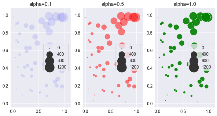
1-2. cmap과 alpha
(1) matplotlib
1 | plt.figure(figsize=(12, 6)) |
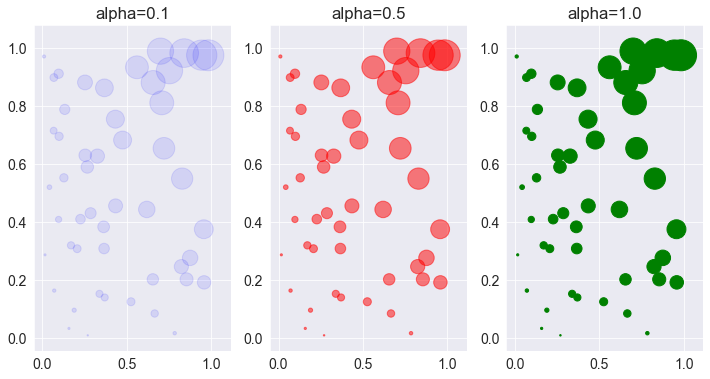
(2) seaborn
1 | plt.figure(figsize=(12, 6)) |
2. Barplot, Barhplot
reference: <sns.barplot> Document
sns.boxplot ( x, y, hue=None, data=None, alpha=‘auto’, palette=None / color=None )
2-1. 기본 Barplot 그리기
(1) matplotlib
1 | x = ['Math', 'Programming', 'Data Science', 'Art', 'English', 'Physics'] |
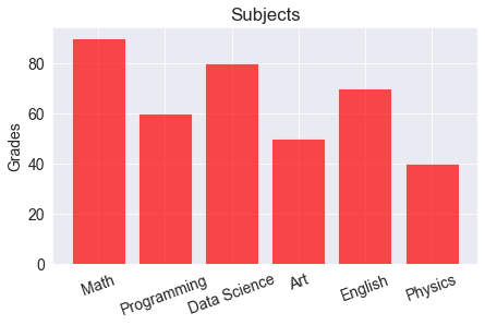
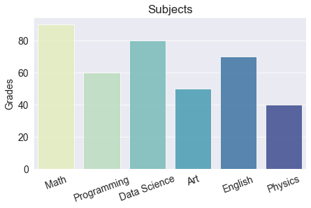
(2) seaborn
1 | x = ['Math', 'Programming', 'Data Science', 'Art', 'English', 'Physics'] |
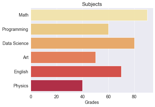
2-2. 기본 Barhplot 그리기
(1) matplotlib
- plt.barh 함수 사용
- bar 함수에서 xticks / ylabel 로 설정했던 부분이 barh 함수에서 yticks / xlabel 로 변경함
1 | x = ['Math', 'Programming', 'Data Science', 'Art', 'English', 'Physics'] |
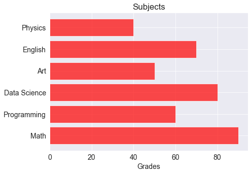
(2) seaborn
- sns.barplot 함수를 그대로 사용
- barplot함수 안에 x와 y의 위치를 교환
xticks설정이 변경 불필요;
하지만 ylabel설정은 xlable로 변경 필요
1 | x = ['Math', 'Programming', 'Data Science', 'Art', 'English', 'Physics'] |
2-3. Barplot에서 비교 그래프 그리기
(1) matplotlib
1 | x_label = ['Math', 'Programming', 'Data Science', 'Art', 'English', 'Physics'] |
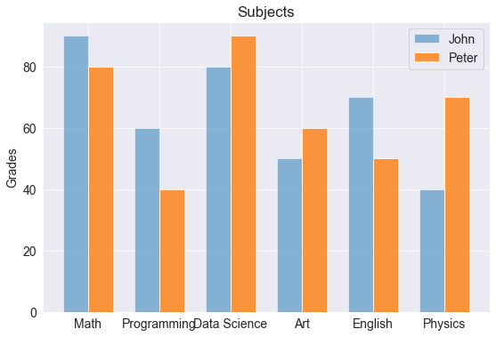
1 | x_label = ['Math', 'Programming', 'Data Science', 'Art', 'English', 'Physics'] |
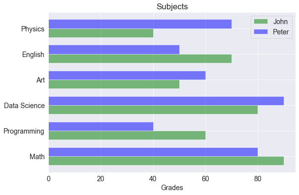
(2) seaborn
Seaborn에서는 위의 matplotlib과 조금 다른 방식을 취한다.
seaborn에서 hue옵션으로 매우 쉽게 비교 barplot을 그릴 수 있음.
sns.barplot ( x, y, hue=…, data=…, palette=… )
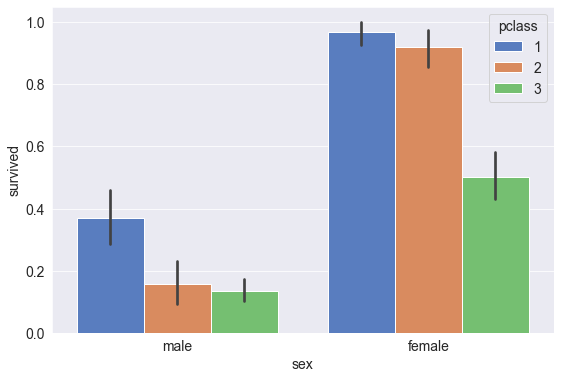
실전 tip.
-
그래프를 임의로 그려야 하는 경우 ->
matplotlib -
DataFrame을 가지고 그리는 경우 ->
seaborn
1 | titanic = sns.load_dataset('titanic') |
| survived | pclass | sex | age | sibsp | parch | fare | embarked | class | who | adult_male | deck | embark_town | alive | alone | |
|---|---|---|---|---|---|---|---|---|---|---|---|---|---|---|---|
| 0 | 0 | 3 | male | 22.0 | 1 | 0 | 7.2500 | S | Third | man | True | NaN | Southampton | no | False |
| 1 | 1 | 1 | female | 38.0 | 1 | 0 | 71.2833 | C | First | woman | False | C | Cherbourg | yes | False |
| 2 | 1 | 3 | female | 26.0 | 0 | 0 | 7.9250 | S | Third | woman | False | NaN | Southampton | yes | True |
| 3 | 1 | 1 | female | 35.0 | 1 | 0 | 53.1000 | S | First | woman | False | C | Southampton | yes | False |
| 4 | 0 | 3 | male | 35.0 | 0 | 0 | 8.0500 | S | Third | man | True | NaN | Southampton | no | True |
1 | sns.barplot(x='sex', y='survived', hue='pclass', data=titanic, palette='muted') |
3. Line Plot
reference: <sns.lineplot> Document
sns.lineplot ( x, y, label=…, color=None, alpha=‘auto’, marker=None, linestyle=None )
- 기본 옵션은 matplotlib의
plt.plot과 비슷- 함수만
plt.plot에서sns.lineplot로 바꾸면 됨- plt.legend() 명령어 따로 쓸 필요없음
- 배경이 whitegrid / darkgrid 로 설정되어 있을 시 plt.grid() 명령어 불필요
3-1. 기본 lineplot 그리기
(1) matplotlib
1 | x = np.arange(0, 10, 0.1) |
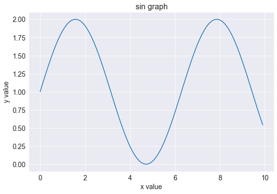
(2) seaborn
1 | sns.lineplot(x, y) # 함수만 변경하면 됨 (plt.plot -> sns.lineplot) |

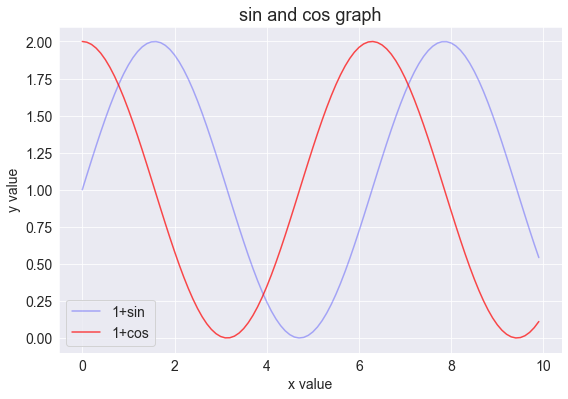
3-2. 2개 이상의 그래프 그리기
1 | x = np.arange(0, 10, 0.1) |
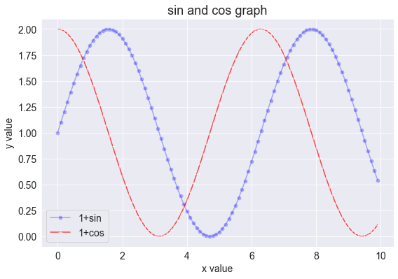
3-3. 마커 스타일링
- marker: 마커 옵션
1 | x = np.arange(0, 10, 0.1) |
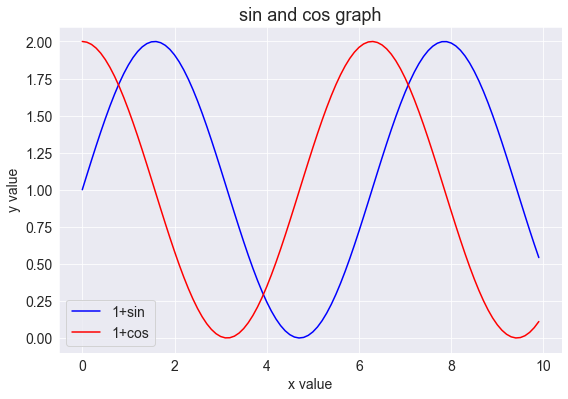
3-4. 라인 스타일 변경하기
- linestyle: 라인 스타일 변경하기
1 | x = np.arange(0, 10, 0.1) |
4. Areaplot (Filled Area)
Seaborn에서는 areaplot을 지원하지 않음
matplotlib을 활용하여 구현해야 함
5.Histogram
reference: <sns.distplot> Document
sns.distplot ( x, bins=None, hist=True, kde=True, vertical=False )
- bins: hist bins 갯수 설정
- hist: Whether to plot a (normed) histogram
- kde: Whether to plot a gaussian kernel density estimate
- vertical: If True, observed values are on y-axis
5-1. 기본 Histogram 그리기
(1) matplotlib
1 | N = 100000 |
(2) seaborn
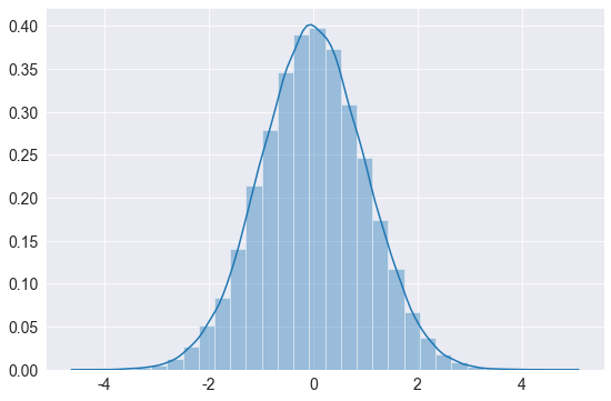
Histogram + Density Function (default)
1 | N = 100000 |
<matplotlib.axes._subplots.AxesSubplot at 0x1ba5cc800c8>
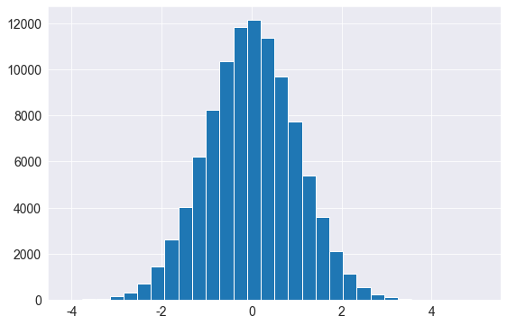
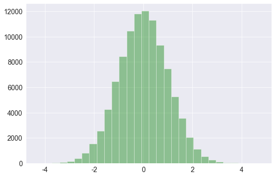
Histogram Only
1 | sns.distplot(x, bins=bins, hist=True, kde=False, color='g') |
<matplotlib.axes._subplots.AxesSubplot at 0x1ba5cd09788>
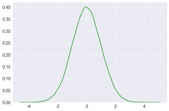
Density Function Only
1 | sns.distplot(x, bins=bins, hist=False, kde=True, color='g') |
<matplotlib.axes._subplots.AxesSubplot at 0x1ba5c7cc208>
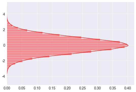
수평 그래프
1 | sns.distplot(x, bins=bins, vertical=True, color='r') |
<matplotlib.axes._subplots.AxesSubplot at 0x1ba5c250108>
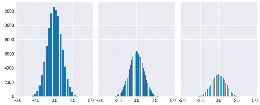
5-2. 다중 Histogram 그리기
matplotlib 에서의 방법을 사용
1 | N = 100000 |
6. Pie Chart
Seaborn에서는 pie plot을 지원하지 않음
matplotlib을 활용하여 구현해야 함
7. Box Plot
reference: <sns.boxplot> Document
sns.baxplot ( x=None, y=None, hue=None, data=None, orient=None, width=0.8 )
- hue: 비교 그래프를 그릴 때 나눔 기준이 되는 Variable 설정
- orient: “v” / “h”. Orientation of the plot (vertical or horizontal)
- width: box의 넓이
7-1. 기본 박스플롯 생성
샘플 데이터 생성
1 | # DGP |
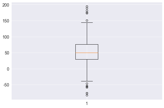
(1) matplotlib
1 | plt.boxplot(data) |
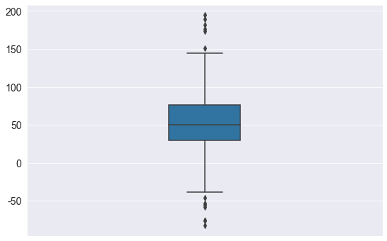
(2) seaborn
1 | sns.boxplot(data, orient='v', width=0.2) |
7-2. 다중 박스플롯 생성
seaborn에서는 hue옵션으로 매우 쉽게 비교 boxplot을 그릴 수 있으며 주로 DataFrame을 가지고 그릴 때 활용한다.
barplot과 마찬가지로, 용도에 따라 적절한 library를 사용한다
실전 Tip.
-
그래프를 임의로 그려야 하는 경우 ->
matplotlit -
DataFrame을 가지고 그리는 경우 ->
seaborn
(1) matplotlib
1 | # DGP |
1 | plt.boxplot(data) |
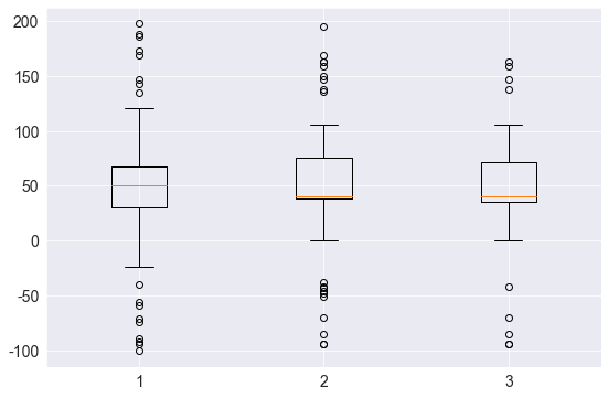
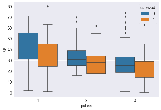
(2) seaborn
1 | titanic = sns.load_dataset('titanic') |
| survived | pclass | sex | age | sibsp | parch | fare | embarked | class | who | adult_male | deck | embark_town | alive | alone | |
|---|---|---|---|---|---|---|---|---|---|---|---|---|---|---|---|
| 0 | 0 | 3 | male | 22.0 | 1 | 0 | 7.2500 | S | Third | man | True | NaN | Southampton | no | False |
| 1 | 1 | 1 | female | 38.0 | 1 | 0 | 71.2833 | C | First | woman | False | C | Cherbourg | yes | False |
| 2 | 1 | 3 | female | 26.0 | 0 | 0 | 7.9250 | S | Third | woman | False | NaN | Southampton | yes | True |
| 3 | 1 | 1 | female | 35.0 | 1 | 0 | 53.1000 | S | First | woman | False | C | Southampton | yes | False |
| 4 | 0 | 3 | male | 35.0 | 0 | 0 | 8.0500 | S | Third | man | True | NaN | Southampton | no | True |
1 | sns.boxplot(x='pclass', y='age', hue='survived', data=titanic) |
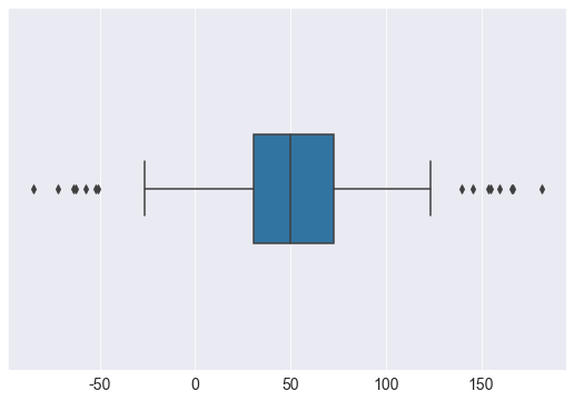
7-3. Box Plot 축 바꾸기
(1) 단일 boxplot
- orient옵션: orient = "h"로 설정
1 | # DGP |
1 | sns.boxplot(data, orient='h', width=0.3) |
<matplotlib.axes._subplots.AxesSubplot at 0x1ba5e866188>
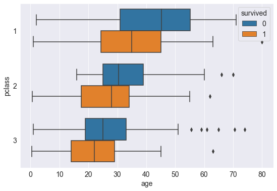
(2) 다중 boxplot
- x, y 변수 교환
- orient = “h”
1 | sns.boxplot(y='pclass', x='age', hue='survived', data=titanic, orient='h') |
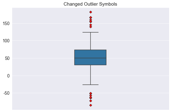
7-4. Outlier 마커 심볼과 컬러 변경
- flierprops = … 옵션 사용 (matplotlib과 동일)
1 | outlier_marker = dict(markerfacecolor='r', marker='D') |