회귀 (Regression) 예측
특성: 수치형 값을 예측 (Y의 값이 연속형 수치로 표현)
예시:
-
주택 가격 예측
-
매출앵 예측
0. 데이터 셋
1 | import pandas as pd |
1 | from sklearn.datasets import load_boston |
0-1. 데이터 로드
1 | data = load_boston() |
1 | print(data['DESCR']) # data description |
.. _boston_dataset:

Boston house prices dataset
---------------------------

**Data Set Characteristics:**

    :Number of Instances: 506

    :Number of Attributes: 13 numeric/categorical predictive. Median Value (attribute 14) is usually the target.

    :Attribute Information (in order):
        - CRIM     per capita crime rate by town
        - ZN       proportion of residential land zoned for lots over 25,000 sq.ft.
        - INDUS    proportion of non-retail business acres per town
        - CHAS     Charles River dummy variable (= 1 if tract bounds river; 0 otherwise)
        - NOX      nitric oxides concentration (parts per 10 million)
        - RM       average number of rooms per dwelling
        - AGE      proportion of owner-occupied units built prior to 1940
        - DIS      weighted distances to five Boston employment centres
        - RAD      index of accessibility to radial highways
        - TAX      full-value property-tax rate per $10,000
        - PTRATIO  pupil-teacher ratio by town
        - B        1000(Bk - 0.63)^2 where Bk is the proportion of blacks by town
        - LSTAT    % lower status of the population
        - MEDV     Median value of owner-occupied homes in $1000's

    :Missing Attribute Values: None

    :Creator: Harrison, D. and Rubinfeld, D.L.

This is a copy of UCI ML housing dataset.
https://archive.ics.uci.edu/ml/machine-learning-databases/housing/
This dataset was taken from the StatLib library which is maintained at Carnegie Mellon University.

The Boston house-price data of Harrison, D. and Rubinfeld, D.L. 'Hedonic
prices and the demand for clean air', J. Environ. Economics & Management,
vol.5, 81-102, 1978.   Used in Belsley, Kuh & Welsch, 'Regression diagnostics
...', Wiley, 1980.   N.B. Various transformations are used in the table on
pages 244-261 of the latter.

The Boston house-price data has been used in many machine learning papers that address regression
problems.

.. topic:: References

   - Belsley, Kuh & Welsch, 'Regression diagnostics: Identifying Influential Data and Sources of Collinearity', Wiley, 1980. 244-261.
   - Quinlan,R. (1993). Combining Instance-Based and Model-Based Learning. In Proceedings on the Tenth International Conference of Machine Learning, 236-243, University of Massachusetts, Amherst. Morgan Kaufmann.
0-2. 데이터프레임 만들기
1 | # step 1. features (X) |
1 | df.head() |
| CRIM | ZN | INDUS | CHAS | NOX | RM | AGE | DIS | RAD | TAX | PTRATIO | B | LSTAT | MEDV | |
|---|---|---|---|---|---|---|---|---|---|---|---|---|---|---|
| 0 | 0.00632 | 18.0 | 2.31 | 0.0 | 0.538 | 6.575 | 65.2 | 4.0900 | 1.0 | 296.0 | 15.3 | 396.90 | 4.98 | 24.0 |
| 1 | 0.02731 | 0.0 | 7.07 | 0.0 | 0.469 | 6.421 | 78.9 | 4.9671 | 2.0 | 242.0 | 17.8 | 396.90 | 9.14 | 21.6 |
| 2 | 0.02729 | 0.0 | 7.07 | 0.0 | 0.469 | 7.185 | 61.1 | 4.9671 | 2.0 | 242.0 | 17.8 | 392.83 | 4.03 | 34.7 |
| 3 | 0.03237 | 0.0 | 2.18 | 0.0 | 0.458 | 6.998 | 45.8 | 6.0622 | 3.0 | 222.0 | 18.7 | 394.63 | 2.94 | 33.4 |
| 4 | 0.06905 | 0.0 | 2.18 | 0.0 | 0.458 | 7.147 | 54.2 | 6.0622 | 3.0 | 222.0 | 18.7 | 396.90 | 5.33 | 36.2 |
컬럼 소게 (feature 13 + target 1):
-
CRIM: 범죄율
-
ZN: 25,000 square feet 당 주거용 토지의 비율
-
INDUS: 비소매(non-retail) 비즈니스 면적 비율
-
CHAS: 찰스 강 더미 변수 (통로가 하천을 향하면 1; 그렇지 않으면 0)
-
NOX: 산화 질소 농도 (천만 분의 1)
-
RM:주거 당 평균 객실 수
-
AGE: 1940 년 이전에 건축된 자가 소유 점유 비율
-
DIS: 5 개의 보스턴 고용 센터까지의 가중 거리
-
RAD: 고속도로 접근성 지수
-
TAX: 10,000 달러 당 전체 가치 재산 세율
-
PTRATIO 도시 별 학생-교사 비율
-
B: 1000 (Bk-0.63) ^ 2 여기서 Bk는 도시 별 검정 비율입니다.
-
LSTAT: 인구의 낮은 지위
-
MEDV: 자가 주택의 중앙값 (1,000 달러 단위)
1. Training set / Test set 나누기
1 | from sklearn.model_selection import train_test_split |
1 | x_train, x_test, y_train, y_test = train_test_split(df.drop('MEDV', 1), df['MEDV'], random_state=23) |
1 | x_train.shape, y_train.shape |
((379, 13), (379,))
1 | x_test.shape, y_test.shape |
((127, 13), (127,))
1 | x_train.head() |
| CRIM | ZN | INDUS | CHAS | NOX | RM | AGE | DIS | RAD | TAX | PTRATIO | B | LSTAT | |
|---|---|---|---|---|---|---|---|---|---|---|---|---|---|
| 112 | 0.12329 | 0.0 | 10.01 | 0.0 | 0.547 | 5.913 | 92.9 | 2.3534 | 6.0 | 432.0 | 17.8 | 394.95 | 16.21 |
| 301 | 0.03537 | 34.0 | 6.09 | 0.0 | 0.433 | 6.590 | 40.4 | 5.4917 | 7.0 | 329.0 | 16.1 | 395.75 | 9.50 |
| 401 | 14.23620 | 0.0 | 18.10 | 0.0 | 0.693 | 6.343 | 100.0 | 1.5741 | 24.0 | 666.0 | 20.2 | 396.90 | 20.32 |
| 177 | 0.05425 | 0.0 | 4.05 | 0.0 | 0.510 | 6.315 | 73.4 | 3.3175 | 5.0 | 296.0 | 16.6 | 395.60 | 6.29 |
| 69 | 0.12816 | 12.5 | 6.07 | 0.0 | 0.409 | 5.885 | 33.0 | 6.4980 | 4.0 | 345.0 | 18.9 | 396.90 | 8.79 |
1 | y_train.head() |
112    18.8
301    22.0
401     7.2
177    24.6
69     20.9
Name: MEDV, dtype: float64
2. 평가 지표 만들기
2-1. 평가 지표 계산식
(1) MAE (Mean Absolute Error)
MAE (평균 절대 오차): 에측값과 실제값의 차이의 절대값에 대하여 평균을 낸 것
(2) MSE (Mean Squared Error)
MSE (평균 제곱 오차): 예측값과 실제값의 차이의 제곱에 대하여 평균을 낸 것
(3) RMSE (Root Mean Squared Error)
RMSE (평균 제곱근 오차): 예측값과 실제값의 차이의 제곱에 대하여 평균을 낸 뒤 루트를 씌운 것
2-2. 코딩으로 평가 지표 만들어 보기
1 | import numpy as np |
1 | actual = np.array([1, 2, 3]) |
1 | # MAE |
2.0
1 | # MSE |
4.0
1 | # RMSE |
2.0
2-3. sklearn의 평가 지표 활용하기
1 | from sklearn.metrics import mean_absolute_error, mean_squared_error |
[sklearn.metrics.mean_absolute_error]
[sklearn.metrics.mean_squared_error]
1 | # MAE (my_mae VS sklearn_mae) |
(2.0, 2.0)
1 | # MSE (my_mse VS sklearn_mse) |
(4.0, 4.0)
2-4. 모델 성능 확인을 위한 함수
1 | import matplotlib.pyplot as plt |
3. 회귀 알고리즘
3-1. Linear Regression
[sklearn.linear_model.LinearRegression] Document
1 | from sklearn.linear_model import LinearRegression |
1 | model = LinearRegression(n_jobs=-1) # n_jobs: CPU코어의 사용 |
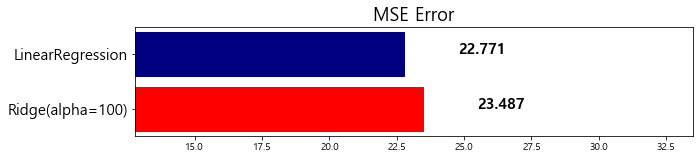
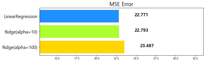
1 | mse_eval('LinearRegression', y_test, pred) |
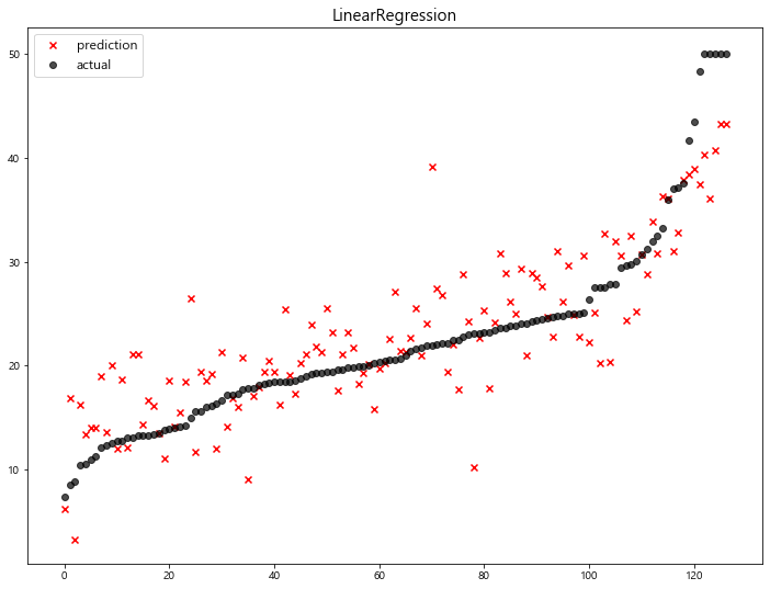
              model        mse
0  LinearRegression  22.770784

3-2. Ridge & LASSO & ElasticNet
(1) 개념
규제(Regularization): 학습이 과적합 되는 것을 방지하고자 일종의 penalty를 부여하는 것.
[원리] penalty를 부여하여 가중치()를 축소함으로써 학습 모델의 예측 variance를 감소 시키는 것
>> L2 규제 & Ridge (릿지)
-
L2 규제 (L2 Regularization): 각 가중치 제곱의 합에 규제 강도 (Regularization Strength) 를 곱한다
-
Ridge: Loss Function에 L2 규제를 더한 값을 최소화 시키는 것
-
를 크게 하면 가중치() 가 더 많이 감소되고(규제를 중요시 함), 를 작게 하면 가중치() 가 증가한다(규제를 중요시하지 않음)
>> L1 규제 & LASSO (라쏘)
-
L1 규제 (L1 Regularization): 각 가중치 절대값의 합에 규제 강도 (Regularization Strength) 를 곱한다
-
LASSO: Loss Function에 L1 규제를 더한 값을 최소화 시키는 것
-
어떤 가중치() 는 실제로 0이 된다. 즉, 모델에서 완전히 제외되는 특성이 생기는 것이다
>> ElasticNet
l1_ratio (default=0.5)
-
l1_ratio = 0 (L2 규제만 사용)
-
l1_ratio = 1 (L1 규제만 사용)
-
0 < l1_ratio <1 (L1 and L2 규제 혼합사용)
(2) 실습
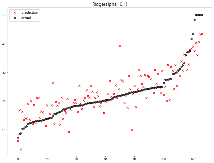
>> Ridge [Document]
1 | from sklearn.linear_model import Ridge |
- 예측 결과 확인
1 | # lambda (규제강도) 범위 설정 |
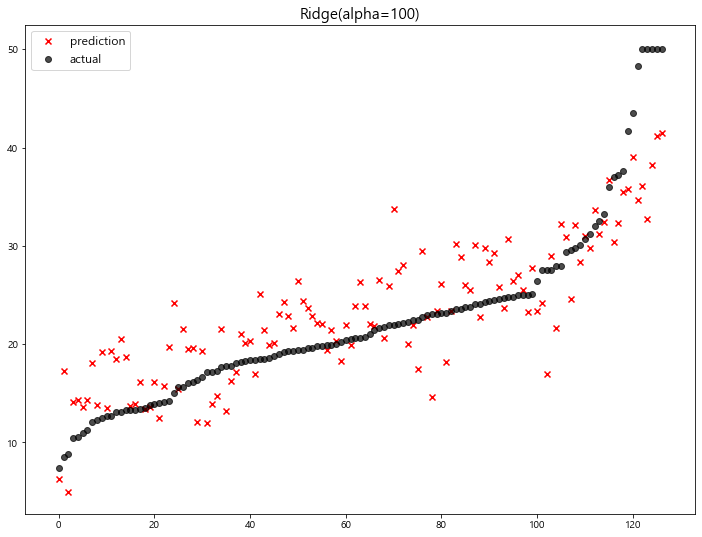
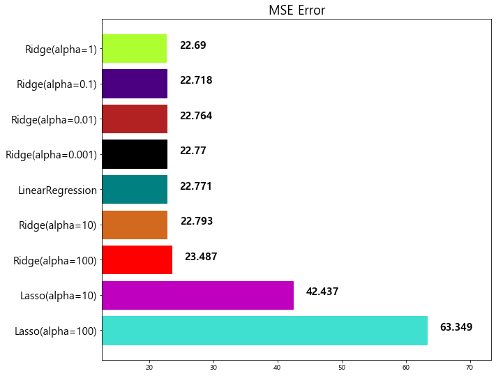
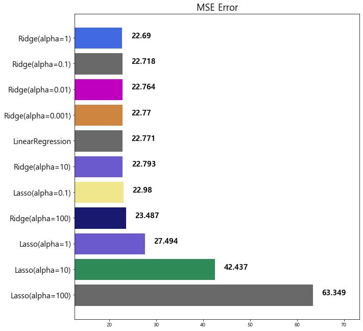
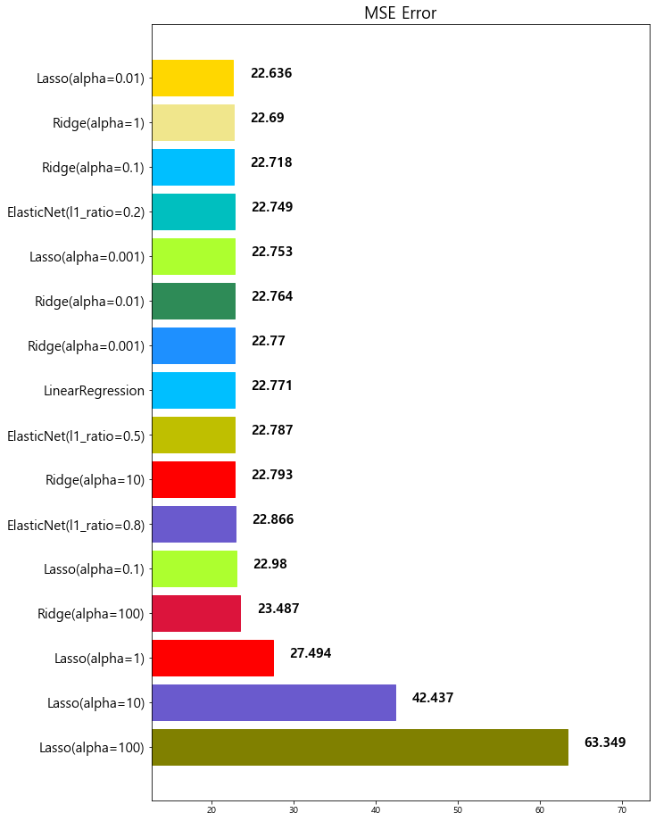
              model        mse
0  Ridge(alpha=100)  23.487453
1  LinearRegression  22.770784
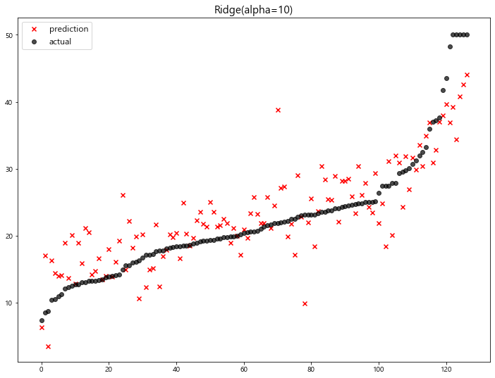
              model        mse
0  Ridge(alpha=100)  23.487453
1   Ridge(alpha=10)  22.793119
2  LinearRegression  22.770784

              model        mse
0  Ridge(alpha=100)  23.487453
1   Ridge(alpha=10)  22.793119
2  LinearRegression  22.770784
3    Ridge(alpha=1)  22.690411
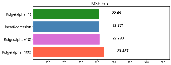
              model        mse
0  Ridge(alpha=100)  23.487453
1   Ridge(alpha=10)  22.793119
2  LinearRegression  22.770784
3  Ridge(alpha=0.1)  22.718126
4    Ridge(alpha=1)  22.690411

model mse
0 Ridge(alpha=100) 23.487453
1 Ridge(alpha=10) 22.793119
2 LinearRegression 22.770784
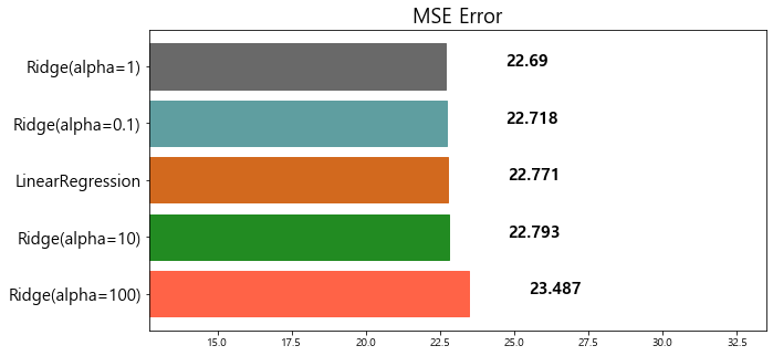
3 Ridge(alpha=0.01) 22.764254
4 Ridge(alpha=0.1) 22.718126
5 Ridge(alpha=1) 22.690411
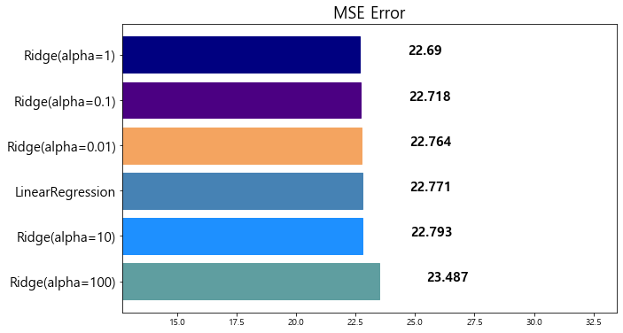

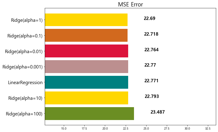
                model        mse
0    Ridge(alpha=100)  23.487453
1     Ridge(alpha=10)  22.793119
2    LinearRegression  22.770784
3  Ridge(alpha=0.001)  22.770117
4   Ridge(alpha=0.01)  22.764254
5    Ridge(alpha=0.1)  22.718126
6      Ridge(alpha=1)  22.690411
- coefficents 값 확인
1 | x_train.columns |
Index(['CRIM', 'ZN', 'INDUS', 'CHAS', 'NOX', 'RM', 'AGE', 'DIS', 'RAD', 'TAX',
       'PTRATIO', 'B', 'LSTAT'],
      dtype='object')
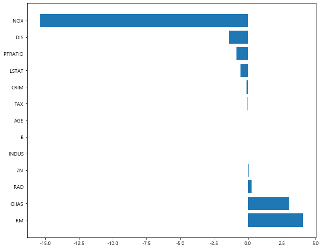
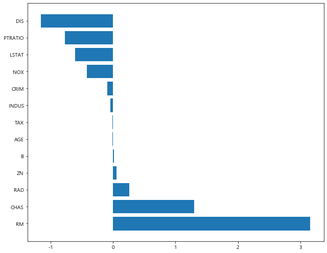
1 | ridge.coef_ # for the last alpha in 'alphas' |
array([ -0.09608448,   0.04753482,   0.0259022 ,   3.24479273,
       -18.89579975,   4.06725732,   0.0020486 ,  -1.46883742,
         0.28149275,  -0.0094656 ,  -0.87454099,   0.01240815,
        -0.52406249])
1 | # coefficients visulization |
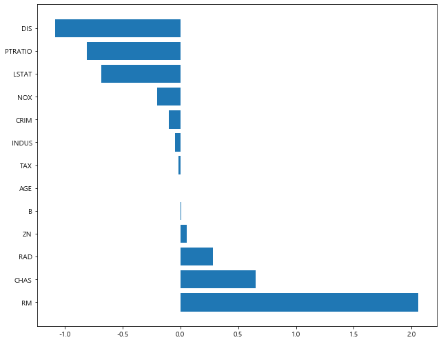
1 | plot_coef(x_train.columns, ridge.coef_) # alpha = 0.001 |
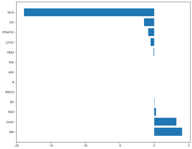
- alpha 값에 따른 coef의 차이
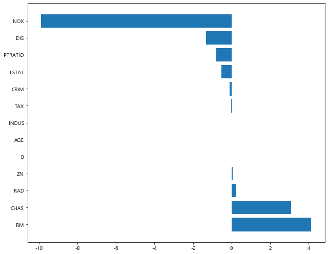
1 | ridge_1 = Ridge(alpha=1) |
1 | plot_coef(x_train.columns, ridge_1.coef_) # alpha = 1 |
1 | plot_coef(x_train.columns, ridge_100.coef_) # alpha = 100 |
>> LASSO [Document]
1 | from sklearn.linear_model import Lasso |
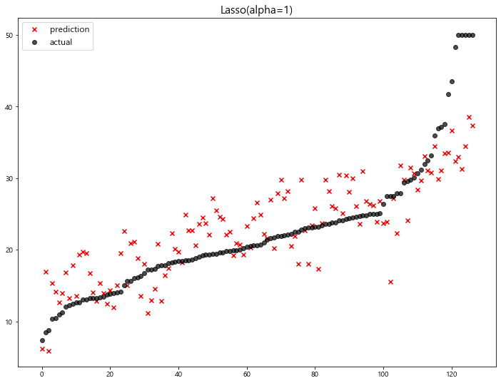
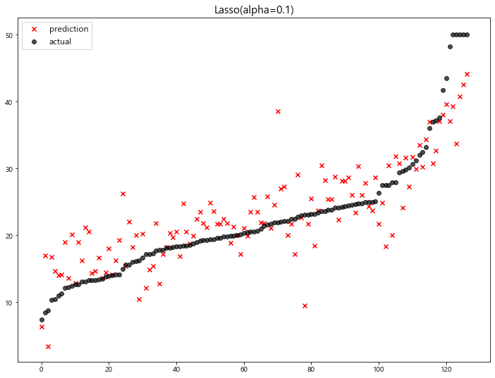
- 예측 결과 확인
1 | # lambda (규제강도) 범위 설정 |
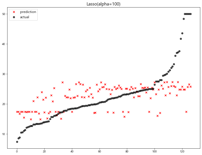
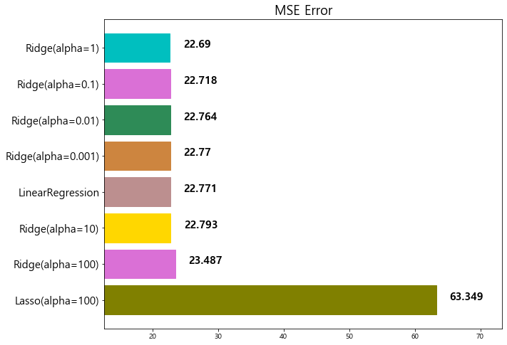
                model        mse
0    Lasso(alpha=100)  63.348818
1    Ridge(alpha=100)  23.487453
2     Ridge(alpha=10)  22.793119
3    LinearRegression  22.770784
4  Ridge(alpha=0.001)  22.770117
5   Ridge(alpha=0.01)  22.764254
6    Ridge(alpha=0.1)  22.718126
7      Ridge(alpha=1)  22.690411
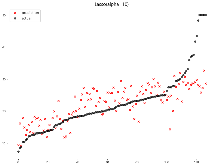
                model        mse
0    Lasso(alpha=100)  63.348818
1     Lasso(alpha=10)  42.436622
2    Ridge(alpha=100)  23.487453
3     Ridge(alpha=10)  22.793119
4    LinearRegression  22.770784
5  Ridge(alpha=0.001)  22.770117
6   Ridge(alpha=0.01)  22.764254
7    Ridge(alpha=0.1)  22.718126
8      Ridge(alpha=1)  22.690411
model mse
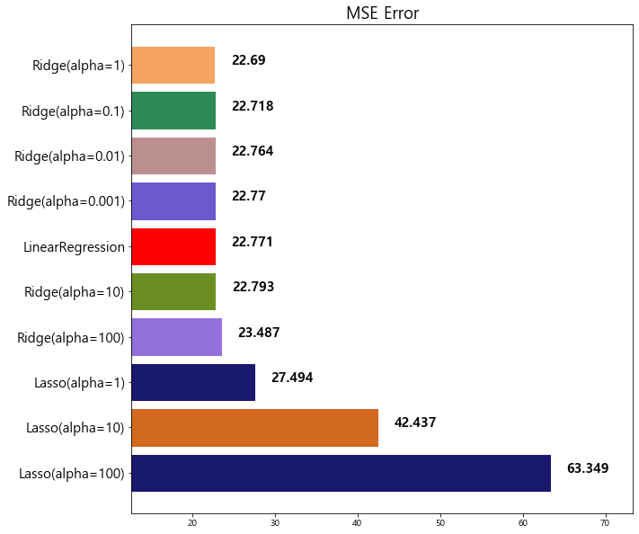
0 Lasso(alpha=100) 63.348818
1 Lasso(alpha=10) 42.436622
2 Lasso(alpha=1) 27.493672
3 Ridge(alpha=100) 23.487453
4 Ridge(alpha=10) 22.793119
5 LinearRegression 22.770784
6 Ridge(alpha=0.001) 22.770117
7 Ridge(alpha=0.01) 22.764254
8 Ridge(alpha=0.1) 22.718126
9 Ridge(alpha=1) 22.690411
                 model        mse
0     Lasso(alpha=100)  63.348818
1      Lasso(alpha=10)  42.436622
2       Lasso(alpha=1)  27.493672
3     Ridge(alpha=100)  23.487453
4     Lasso(alpha=0.1)  22.979708
5      Ridge(alpha=10)  22.793119
6     LinearRegression  22.770784
7   Ridge(alpha=0.001)  22.770117
8    Ridge(alpha=0.01)  22.764254
9     Ridge(alpha=0.1)  22.718126
10      Ridge(alpha=1)  22.690411
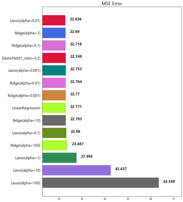
11   Lasso(alpha=0.01)  22.635614

                 model        mse
0     Lasso(alpha=100)  63.348818
1      Lasso(alpha=10)  42.436622
2       Lasso(alpha=1)  27.493672
3     Ridge(alpha=100)  23.487453
4     Lasso(alpha=0.1)  22.979708
5      Ridge(alpha=10)  22.793119
6     LinearRegression  22.770784
7   Ridge(alpha=0.001)  22.770117
8    Ridge(alpha=0.01)  22.764254
9   Lasso(alpha=0.001)  22.753017
10    Ridge(alpha=0.1)  22.718126
11      Ridge(alpha=1)  22.690411
12   Lasso(alpha=0.01)  22.635614
- coefficients 값 확인
1 | # alpha = 0.01 |
[alpha = 0.01]
1 | x_train.columns |
Index(['CRIM', 'ZN', 'INDUS', 'CHAS', 'NOX', 'RM', 'AGE', 'DIS', 'RAD', 'TAX',
       'PTRATIO', 'B', 'LSTAT'],
      dtype='object')
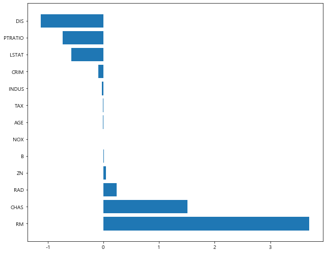
1 | lasso_01.coef_ |
array([ -0.09427142,   0.04759954,   0.01255668,   3.08256139,
       -15.36800113,   4.07373679,  -0.00100439,  -1.40819927,
         0.27152905,  -0.0097157 ,  -0.84377679,   0.01249204,
        -0.52790174])
1 | plot_coef(x_train.columns, lasso_01.coef_) |
[alpha = 100]
1 | x_train.columns |
Index(['CRIM', 'ZN', 'INDUS', 'CHAS', 'NOX', 'RM', 'AGE', 'DIS', 'RAD', 'TAX',
       'PTRATIO', 'B', 'LSTAT'],
      dtype='object')
1 | lasso_100.coef_ |
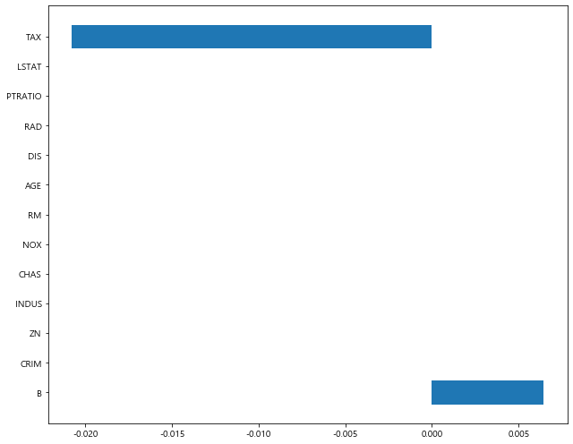
array([-0.        ,  0.        , -0.        ,  0.        , -0.        ,
        0.        , -0.        ,  0.        , -0.        , -0.02078349,
       -0.        ,  0.00644409, -0.        ])
1 | plot_coef(x_train.columns, lasso_100.coef_) |
>> ElasticNet [Document]
1 | from sklearn.linear_model import ElasticNet |
- 예측 결과 확인
1 | ratios = [0.2, 0.5, 0.8] |
1 | # alpha = 0.5 로 고정 |

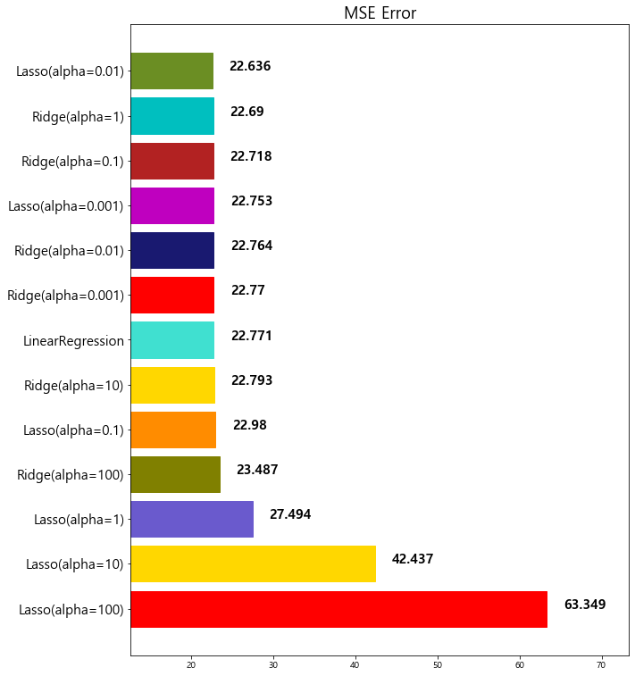
                       model        mse
0           Lasso(alpha=100)  63.348818
1            Lasso(alpha=10)  42.436622
2             Lasso(alpha=1)  27.493672
3           Ridge(alpha=100)  23.487453
4           Lasso(alpha=0.1)  22.979708
5            Ridge(alpha=10)  22.793119
6           LinearRegression  22.770784
7         Ridge(alpha=0.001)  22.770117
8          Ridge(alpha=0.01)  22.764254
9         Lasso(alpha=0.001)  22.753017
10  ElasticNet(l1_ratio=0.2)  22.749018
11          Ridge(alpha=0.1)  22.718126
12            Ridge(alpha=1)  22.690411
13         Lasso(alpha=0.01)  22.635614

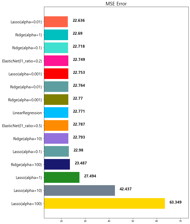
                       model        mse
0           Lasso(alpha=100)  63.348818
1            Lasso(alpha=10)  42.436622
2             Lasso(alpha=1)  27.493672
3           Ridge(alpha=100)  23.487453
4           Lasso(alpha=0.1)  22.979708
5            Ridge(alpha=10)  22.793119
6   ElasticNet(l1_ratio=0.5)  22.787269
7           LinearRegression  22.770784
8         Ridge(alpha=0.001)  22.770117
9          Ridge(alpha=0.01)  22.764254
10        Lasso(alpha=0.001)  22.753017
11  ElasticNet(l1_ratio=0.2)  22.749018
12          Ridge(alpha=0.1)  22.718126
13            Ridge(alpha=1)  22.690411
14         Lasso(alpha=0.01)  22.635614
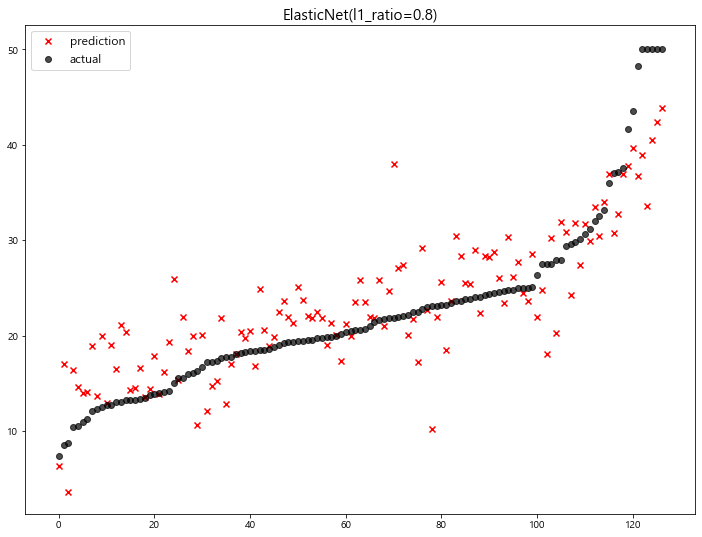
                       model        mse
0           Lasso(alpha=100)  63.348818
1            Lasso(alpha=10)  42.436622
2             Lasso(alpha=1)  27.493672
3           Ridge(alpha=100)  23.487453
4           Lasso(alpha=0.1)  22.979708
5   ElasticNet(l1_ratio=0.8)  22.865628
6            Ridge(alpha=10)  22.793119
7   ElasticNet(l1_ratio=0.5)  22.787269
8           LinearRegression  22.770784
9         Ridge(alpha=0.001)  22.770117
10         Ridge(alpha=0.01)  22.764254
11        Lasso(alpha=0.001)  22.753017
12  ElasticNet(l1_ratio=0.2)  22.749018
13          Ridge(alpha=0.1)  22.718126
14            Ridge(alpha=1)  22.690411
15         Lasso(alpha=0.01)  22.635614
- coefficients 값 확인
1 | # ㅣ1_ratio = 0.2 |
[ l1_ratio = 0.2 ]
1 | x_train.columns |
Index(['CRIM', 'ZN', 'INDUS', 'CHAS', 'NOX', 'RM', 'AGE', 'DIS', 'RAD', 'TAX',
       'PTRATIO', 'B', 'LSTAT'],
      dtype='object')
1 | elasticnet_2.coef_ |
array([-0.09297585,  0.05293361, -0.03950412,  1.30126199, -0.41996826,
        3.15838796, -0.00644646, -1.15290012,  0.25973467, -0.01231233,
       -0.77186571,  0.01201684, -0.60780037])
1 | plot_coef(x_train.columns, elasticnet_2.coef_) |
[ l1_ratio = 0.8 ]
1 | x_train.columns |
Index(['CRIM', 'ZN', 'INDUS', 'CHAS', 'NOX', 'RM', 'AGE', 'DIS', 'RAD', 'TAX',
       'PTRATIO', 'B', 'LSTAT'],
      dtype='object')
1 | elasticnet_8.coef_ |
array([-0.08797633,  0.05035601, -0.03058513,  1.51071961, -0.        ,
        3.70247373, -0.01017259, -1.12431077,  0.24389841, -0.01189981,
       -0.73481448,  0.01259147, -0.573733  ])
1 | plot_coef(x_train.columns, elasticnet_8.coef_) |
4. Scaling
4-1. Scaler 소개
-
StandardScaler
-
MinMaxScaler
-
RobustScaler
1 | from sklearn.preprocessing import StandardScaler, MinMaxScaler, RobustScaler |
1 | x_train.describe() |
| CRIM | ZN | INDUS | CHAS | NOX | RM | AGE | DIS | RAD | TAX | PTRATIO | B | LSTAT | |
|---|---|---|---|---|---|---|---|---|---|---|---|---|---|
| count | 379.000000 | 379.000000 | 379.000000 | 379.000000 | 379.000000 | 379.000000 | 379.000000 | 379.000000 | 379.000000 | 379.000000 | 379.000000 | 379.000000 | 379.000000 |
| mean | 3.512192 | 11.779683 | 10.995013 | 0.076517 | 0.548712 | 6.266953 | 67.223483 | 3.917811 | 9.282322 | 404.680739 | 18.448549 | 357.048100 | 12.633773 |
| std | 8.338717 | 23.492842 | 6.792065 | 0.266175 | 0.115006 | 0.681796 | 28.563787 | 2.084167 | 8.583051 | 166.813256 | 2.154917 | 92.745266 | 7.259213 |
| min | 0.006320 | 0.000000 | 0.460000 | 0.000000 | 0.385000 | 3.561000 | 2.900000 | 1.129600 | 1.000000 | 188.000000 | 12.600000 | 2.520000 | 1.730000 |
| 25% | 0.078910 | 0.000000 | 5.190000 | 0.000000 | 0.445000 | 5.876500 | 42.250000 | 2.150900 | 4.000000 | 278.000000 | 17.150000 | 375.425000 | 6.910000 |
| 50% | 0.228760 | 0.000000 | 9.690000 | 0.000000 | 0.532000 | 6.208000 | 74.400000 | 3.414500 | 5.000000 | 330.000000 | 19.000000 | 392.110000 | 11.380000 |
| 75% | 2.756855 | 19.000000 | 18.100000 | 0.000000 | 0.624000 | 6.611000 | 93.850000 | 5.400900 | 8.000000 | 666.000000 | 20.200000 | 396.260000 | 16.580000 |
| max | 73.534100 | 100.000000 | 27.740000 | 1.000000 | 0.871000 | 8.398000 | 100.000000 | 10.585700 | 24.000000 | 711.000000 | 22.000000 | 396.900000 | 37.970000 |
>> StandardScaler
평균(mean)을 0, 표준편차(std)를 1로 만들어 주는 scaler
1 | std_scaler = StandardScaler() |
| 0 | 1 | 2 | 3 | 4 | 5 | 6 | 7 | 8 | 9 | 10 | 11 | 12 | |
|---|---|---|---|---|---|---|---|---|---|---|---|---|---|
| count | 379.00 | 379.00 | 379.00 | 379.00 | 379.00 | 379.00 | 379.00 | 379.00 | 379.00 | 379.00 | 379.00 | 379.00 | 379.00 |
| mean | -0.00 | 0.00 | 0.00 | -0.00 | -0.00 | -0.00 | -0.00 | 0.00 | -0.00 | 0.00 | 0.00 | 0.00 | 0.00 |
| std | 1.00 | 1.00 | 1.00 | 1.00 | 1.00 | 1.00 | 1.00 | 1.00 | 1.00 | 1.00 | 1.00 | 1.00 | 1.00 |
| min | -0.42 | -0.50 | -1.55 | -0.29 | -1.43 | -3.97 | -2.25 | -1.34 | -0.97 | -1.30 | -2.72 | -3.83 | -1.50 |
| 25% | -0.41 | -0.50 | -0.86 | -0.29 | -0.90 | -0.57 | -0.88 | -0.85 | -0.62 | -0.76 | -0.60 | 0.20 | -0.79 |
| 50% | -0.39 | -0.50 | -0.19 | -0.29 | -0.15 | -0.09 | 0.25 | -0.24 | -0.50 | -0.45 | 0.26 | 0.38 | -0.17 |
| 75% | -0.09 | 0.31 | 1.05 | -0.29 | 0.66 | 0.51 | 0.93 | 0.71 | -0.15 | 1.57 | 0.81 | 0.42 | 0.54 |
| max | 8.41 | 3.76 | 2.47 | 3.47 | 2.81 | 3.13 | 1.15 | 3.20 | 1.72 | 1.84 | 1.65 | 0.43 | 3.49 |
>> MinMaxScaler
min값과 max값을 0~1사이로 정규화 (Normalize)
1 | minmax_scaler = MinMaxScaler() |
| 0 | 1 | 2 | 3 | 4 | 5 | 6 | 7 | 8 | 9 | 10 | 11 | 12 | |
|---|---|---|---|---|---|---|---|---|---|---|---|---|---|
| count | 379.00 | 379.00 | 379.00 | 379.00 | 379.00 | 379.00 | 379.00 | 379.00 | 379.00 | 379.00 | 379.00 | 379.00 | 379.00 |
| mean | 0.05 | 0.12 | 0.39 | 0.08 | 0.34 | 0.56 | 0.66 | 0.29 | 0.36 | 0.41 | 0.62 | 0.90 | 0.30 |
| std | 0.11 | 0.23 | 0.25 | 0.27 | 0.24 | 0.14 | 0.29 | 0.22 | 0.37 | 0.32 | 0.23 | 0.24 | 0.20 |
| min | 0.00 | 0.00 | 0.00 | 0.00 | 0.00 | 0.00 | 0.00 | 0.00 | 0.00 | 0.00 | 0.00 | 0.00 | 0.00 |
| 25% | 0.00 | 0.00 | 0.17 | 0.00 | 0.12 | 0.48 | 0.41 | 0.11 | 0.13 | 0.17 | 0.48 | 0.95 | 0.14 |
| 50% | 0.00 | 0.00 | 0.34 | 0.00 | 0.30 | 0.55 | 0.74 | 0.24 | 0.17 | 0.27 | 0.68 | 0.99 | 0.27 |
| 75% | 0.04 | 0.19 | 0.65 | 0.00 | 0.49 | 0.63 | 0.94 | 0.45 | 0.30 | 0.91 | 0.81 | 1.00 | 0.41 |
| max | 1.00 | 1.00 | 1.00 | 1.00 | 1.00 | 1.00 | 1.00 | 1.00 | 1.00 | 1.00 | 1.00 | 1.00 | 1.00 |
>> RobustScaler
중앙값(median)이 0, IQR(interquartile rage)이 1이 되도록 변환
outlier 처리에 유용
1 | robust_scaler = RobustScaler() |
0     0.0
1     0.0
2     0.0
3     0.0
4     0.0
5     0.0
6     0.0
7     0.0
8     0.0
9     0.0
10    0.0
11    0.0
12    0.0
dtype: float64
4-2. Scaling 후 모델 학습 – 파이프라인 활용
1 | from sklearn.pipeline import make_pipeline |
1 | # elasticnet(alpha=0.1, l1_ratio=0.2) < without standard scaling > |

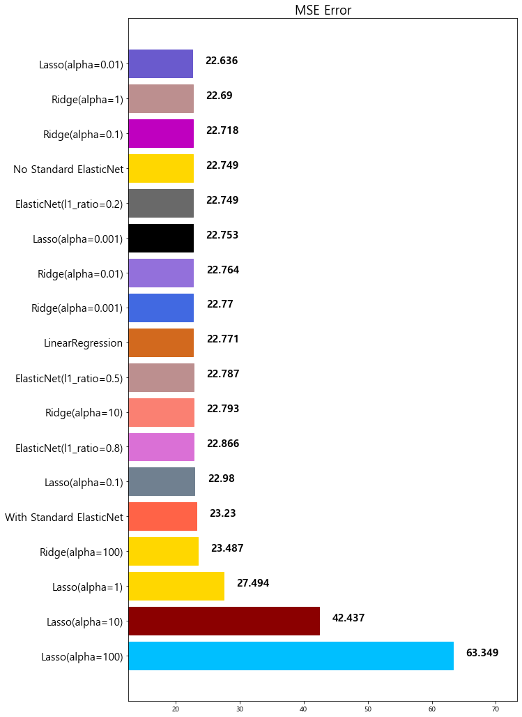
                       model        mse
0           Lasso(alpha=100)  63.348818
1            Lasso(alpha=10)  42.436622
2             Lasso(alpha=1)  27.493672
3           Ridge(alpha=100)  23.487453
4           Lasso(alpha=0.1)  22.979708
5   ElasticNet(l1_ratio=0.8)  22.865628
6            Ridge(alpha=10)  22.793119
7   ElasticNet(l1_ratio=0.5)  22.787269
8           LinearRegression  22.770784
9         Ridge(alpha=0.001)  22.770117
10         Ridge(alpha=0.01)  22.764254
11        Lasso(alpha=0.001)  22.753017
12  ElasticNet(l1_ratio=0.2)  22.749018
13    No Standard ElasticNet  22.749018
14          Ridge(alpha=0.1)  22.718126
15            Ridge(alpha=1)  22.690411
16         Lasso(alpha=0.01)  22.635614
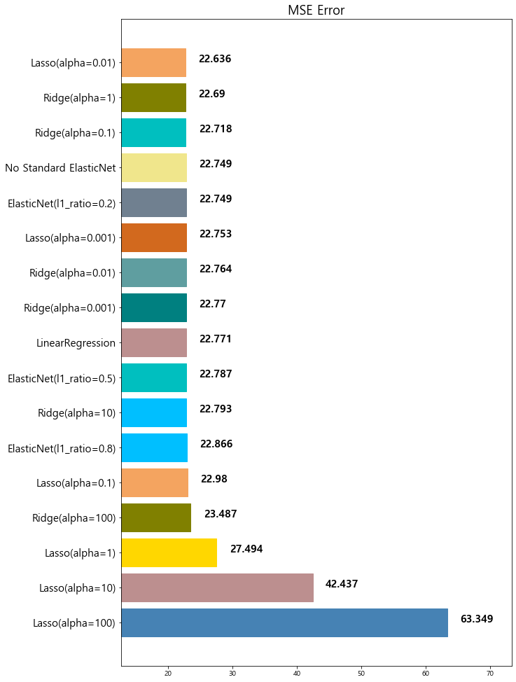
model mse
0 Lasso(alpha=100) 63.348818
1 Lasso(alpha=10) 42.436622
2 Lasso(alpha=1) 27.493672
3 Ridge(alpha=100) 23.487453
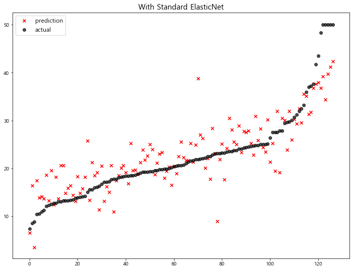
4 With Standard ElasticNet 23.230164
5 Lasso(alpha=0.1) 22.979708
6 ElasticNet(l1_ratio=0.8) 22.865628
7 Ridge(alpha=10) 22.793119
8 ElasticNet(l1_ratio=0.5) 22.787269
9 LinearRegression 22.770784
10 Ridge(alpha=0.001) 22.770117
11 Ridge(alpha=0.01) 22.764254
12 Lasso(alpha=0.001) 22.753017
13 ElasticNet(l1_ratio=0.2) 22.749018
14 No Standard ElasticNet 22.749018
15 Ridge(alpha=0.1) 22.718126
16 Ridge(alpha=1) 22.690411
17 Lasso(alpha=0.01) 22.635614
5. Polynomial Features
다항식의 계수간 상호작용을 통해 새로운 feature를 생성한다.
예를 들면, [a, b] 2개의 feature가 존재한다고 가정하고,
degree=2로 설정한다면, polynomial features 는 [1, a, b, a^2, ab, b^2]가 돤다
1 | from sklearn.preprocessing import PolynomialFeatures |
Polynomial Features 생성
1 | poly = PolynomialFeatures(degree=2, include_bias=False) |
1 | poly_features = poly.fit_transform(x_train)[0] |
array([     0.12329   ,      0.        ,     10.01      ,      0.        ,
            0.547     ,      5.913     ,     92.9       ,      2.3534    ,
            6.        ,    432.        ,     17.8       ,    394.95      ,
           16.21      ,      0.01520042,      0.        ,      1.2341329 ,
            0.        ,      0.06743963,      0.72901377,     11.453641  ,
            0.29015069,      0.73974   ,     53.26128   ,      2.194562  ,
           48.6933855 ,      1.9985309 ,      0.        ,      0.        ,
            0.        ,      0.        ,      0.        ,      0.        ,
            0.        ,      0.        ,      0.        ,      0.        ,
            0.        ,      0.        ,    100.2001    ,      0.        ,
            5.47547   ,     59.18913   ,    929.929     ,     23.557534  ,
           60.06      ,   4324.32      ,    178.178     ,   3953.4495    ,
          162.2621    ,      0.        ,      0.        ,      0.        ,
            0.        ,      0.        ,      0.        ,      0.        ,
            0.        ,      0.        ,      0.        ,      0.299209  ,
            3.234411  ,     50.8163    ,      1.2873098 ,      3.282     ,
          236.304     ,      9.7366    ,    216.03765   ,      8.86687   ,
           34.963569  ,    549.3177    ,     13.9156542 ,     35.478     ,
         2554.416     ,    105.2514    ,   2335.33935   ,     95.84973   ,
         8630.41      ,    218.63086   ,    557.4       ,  40132.8       ,
         1653.62      ,  36690.855     ,   1505.909     ,      5.53849156,
           14.1204    ,   1016.6688    ,     41.89052   ,    929.47533   ,
           38.148614  ,     36.        ,   2592.        ,    106.8       ,
         2369.7       ,     97.26      , 186624.        ,   7689.6       ,
       170618.4       ,   7002.72      ,    316.84      ,   7030.11      ,
          288.538     , 155985.5025    ,   6402.1395    ,    262.7641    ])
1 | x_train.iloc[0] |
CRIM         0.12329
ZN           0.00000
INDUS       10.01000
CHAS         0.00000
NOX          0.54700
RM           5.91300
AGE         92.90000
DIS          2.35340
RAD          6.00000
TAX        432.00000
PTRATIO     17.80000
B          394.95000
LSTAT       16.21000
Name: 112, dtype: float64
Polynomial Features + Standard Scaling 후 모델 학습
1 | poly_pipeline = make_pipeline( |
1 | poly_pred = poly_pipeline.fit(x_train, y_train).predict(x_test) |
D:\Anaconda\lib\site-packages\sklearn\linear_model\_coordinate_descent.py:476: ConvergenceWarning: Objective did not converge. You might want to increase the number of iterations. Duality gap: 32.61172784964583, tolerance: 3.2374824854881266
  positive)
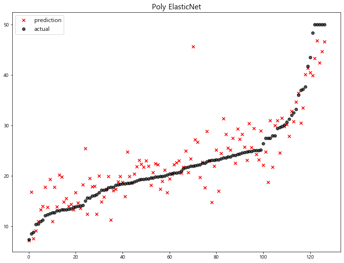
1 | mse_eval('Poly ElasticNet', y_test, poly_pred) |
                       model        mse
0           Lasso(alpha=100)  63.348818
1            Lasso(alpha=10)  42.436622
2             Lasso(alpha=1)  27.493672
3           Ridge(alpha=100)  23.487453
4   With Standard ElasticNet  23.230164
5           Lasso(alpha=0.1)  22.979708
6   ElasticNet(l1_ratio=0.8)  22.865628
7            Ridge(alpha=10)  22.793119
8   ElasticNet(l1_ratio=0.5)  22.787269
9           LinearRegression  22.770784
10        Ridge(alpha=0.001)  22.770117
11         Ridge(alpha=0.01)  22.764254
12        Lasso(alpha=0.001)  22.753017
13  ElasticNet(l1_ratio=0.2)  22.749018
14    No Standard ElasticNet  22.749018
15          Ridge(alpha=0.1)  22.718126
16            Ridge(alpha=1)  22.690411
17         Lasso(alpha=0.01)  22.635614
18           Poly ElasticNet  17.526214
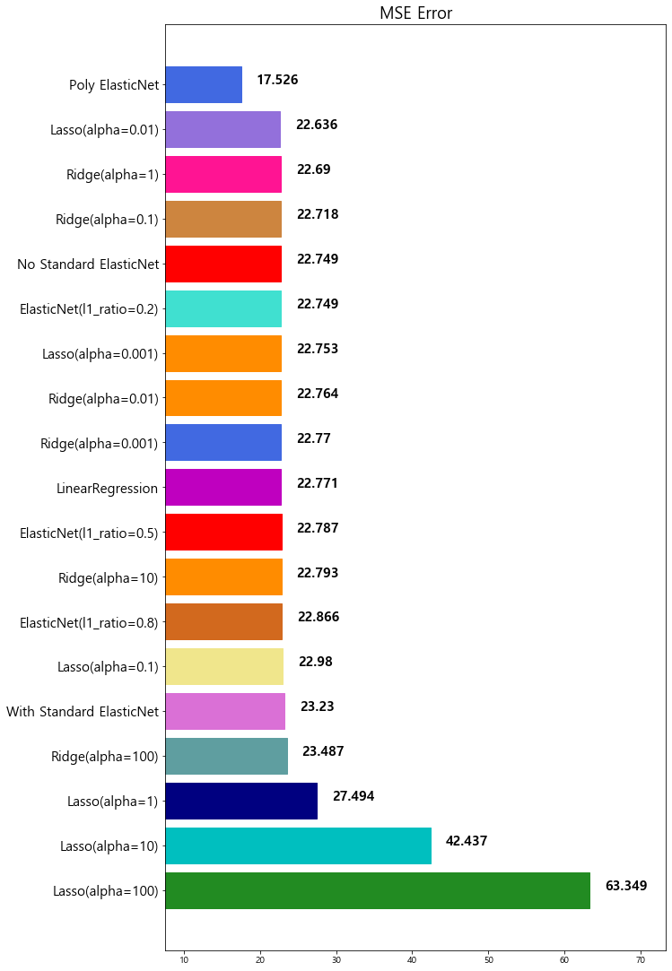
2차 Polynomial Features 추가 후 학습된 모델의 성능이 많이 향상 된것을 확인할 수 있다