.. _iris_dataset:
Iris plants dataset
--------------------
**Data Set Characteristics:**
:Number of Instances: 150 (50 in each of three classes)
:Number of Attributes: 4 numeric, predictive attributes and the class
:Attribute Information:
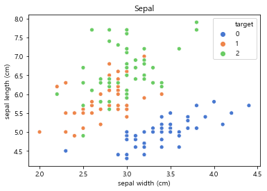
- sepal length in cm
- sepal width in cm
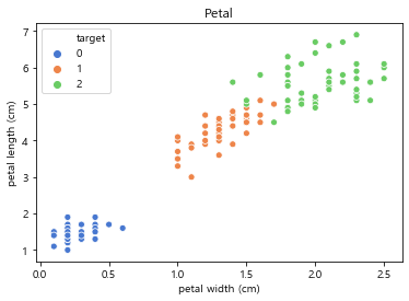
- petal length in cm
- petal width in cm
- class:
- Iris-Setosa
- Iris-Versicolour
- Iris-Virginica
:Summary Statistics:
============== ==== ==== ======= ===== ====================
Min Max Mean SD Class Correlation
============== ==== ==== ======= ===== ====================
sepal length: 4.3 7.9 5.84 0.83 0.7826
sepal width: 2.0 4.4 3.05 0.43 -0.4194
petal length: 1.0 6.9 3.76 1.76 0.9490 (high!)
petal width: 0.1 2.5 1.20 0.76 0.9565 (high!)
============== ==== ==== ======= ===== ====================
:Missing Attribute Values: None
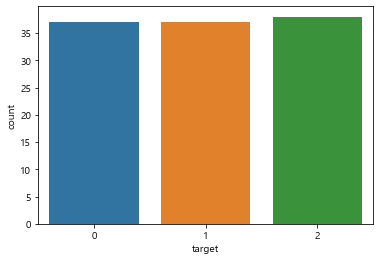
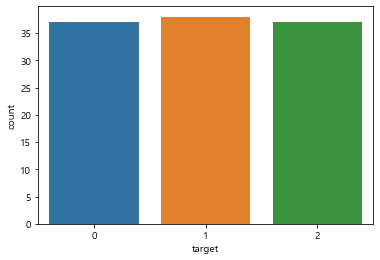
:Class Distribution: 33.3% for each of 3 classes.
:Creator: R.A. Fisher
:Donor: Michael Marshall (MARSHALL%PLU@io.arc.nasa.gov)
:Date: July, 1988
The famous Iris database, first used by Sir R.A. Fisher. The dataset is taken
from Fisher's paper. Note that it's the same as in R, but not as in the UCI
Machine Learning Repository, which has two wrong data points.
This is perhaps the best known database to be found in the
pattern recognition literature. Fisher's paper is a classic in the field and
is referenced frequently to this day. (See Duda & Hart, for example.) The
data set contains 3 classes of 50 instances each, where each class refers to a
type of iris plant. One class is linearly separable from the other 2; the
latter are NOT linearly separable from each other.
.. topic:: References
- Fisher, R.A. "The use of multiple measurements in taxonomic problems"
Annual Eugenics, 7, Part II, 179-188 (1936); also in "Contributions to
Mathematical Statistics" (John Wiley, NY, 1950).
- Duda, R.O., & Hart, P.E. (1973) Pattern Classification and Scene Analysis.
(Q327.D83) John Wiley & Sons. ISBN 0-471-22361-1. See page 218.
- Dasarathy, B.V. (1980) "Nosing Around the Neighborhood: A New System
Structure and Classification Rule for Recognition in Partially Exposed
Environments". IEEE Transactions on Pattern Analysis and Machine
Intelligence, Vol. PAMI-2, No. 1, 67-71.
- Gates, G.W. (1972) "The Reduced Nearest Neighbor Rule". IEEE Transactions
on Information Theory, May 1972, 431-433.
- See also: 1988 MLC Proceedings, 54-64. Cheeseman et al"s AUTOCLASS II
conceptual clustering system finds 3 classes in the data.
- Many, many more ...
<matplotlib.axes._subplots.AxesSubplot at 0x1cb7aaaeec8>
'target’값이 0, 1, 2인 데이터가 Original dataset으로 부터 랜덤으로 뽑히기 때문에 비율의 차이가 존재할 수 있다. 따라서 기계학습할 때 sample size가 큰 데이터 위주로 학습하여 모델의 예측성능이 떨어질 수 있다. (위 상황에서, 학습된 머신러닝 모델이 sample size가 큰 target=1인 경우를 좀 더 잘 예측하고, target=2에 대한 예측도가 떨어질 수 있다)
이를 방지하기 위해 우리는 stratify옵션을 이용하여 label의 class 분포를 균등하게 배분한다.
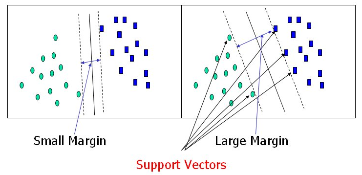
Logistic Regression, SVM(Support Vector Machine)과 같은 알고리즘은 이진(Binary Class) 분류만 가능한다. (2개의 클래스 판별만 가능한다.)
하지만, 3개 이상의 클래스에 대한 판별 **[다중 클래스(Multi-Class) 분류]**을 진행하는 경우, 다음과 같은 전략으로 판별한다.
one-vs-one (OvO): K 개의 클래스가 존재할 때, 이 중 2개의 클래스 조합을 선택하여 K(K−1)/2 개의 이진 클래스 분류 문제를 풀고 이진판별을 통해 가장 많은 판별값을 얻은 클래스를 선택하는 방법이다.
one-vs-rest (OvR): K 개의 클래스가 존재할 때, 클래스들을 “k번째 클래스(one)” & "나머지(rest)"로 나누어서 K개의 개별 이진 분류 문제를 푼다. 즉, 각각의 클래스에 대해 표본이 속하는지(y=1) 속하지 않는지(y=0)의 이진 분류 문제를 푸는 것이다. OvO와 달리 클래스 수만큼의 이진 분류 문제를 풀면 된다.
대부분 OvsR 전략을 선호합니다.
1
from sklearn.linear_model import LogisticRegression
Collecting pydotNote: you may need to restart the kernel to use updated packages.
Downloading pydot-1.4.1-py2.py3-none-any.whl (19 kB)
Requirement already satisfied: pyparsing>=2.1.4 in d:\anaconda\lib\site-packages (from pydot) (2.4.6)
Installing collected packages: pydot
Successfully installed pydot-1.4.1
Requirement already up-to-date: graphviz in d:\anaconda\lib\site-packages (0.14.1)
Note: you may need to restart the kernel to use updated packages.
1
import graphviz
1 2 3 4 5 6
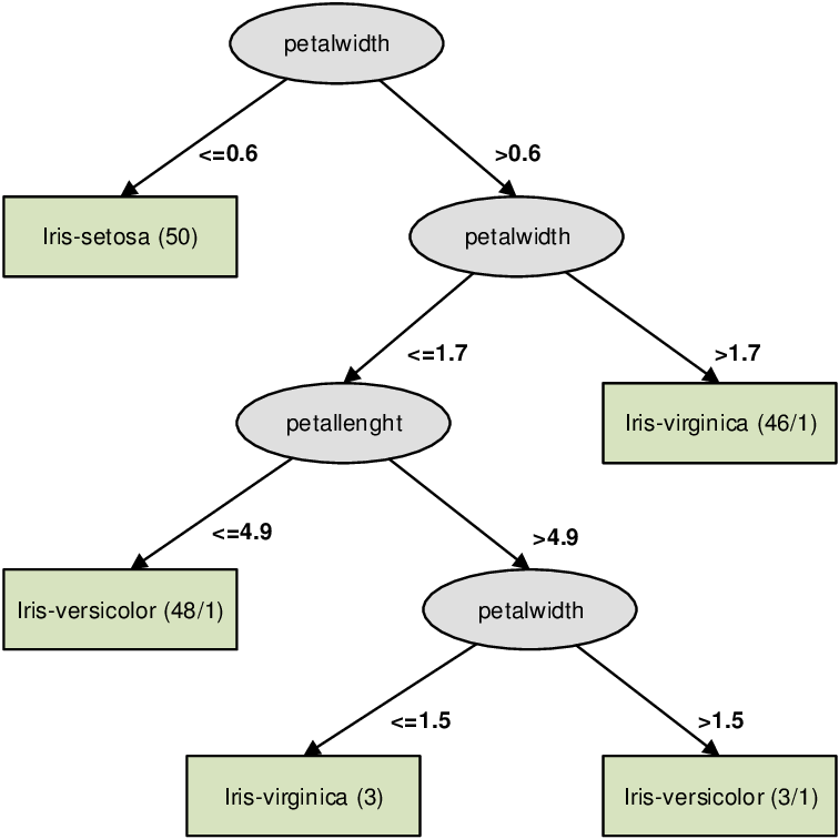
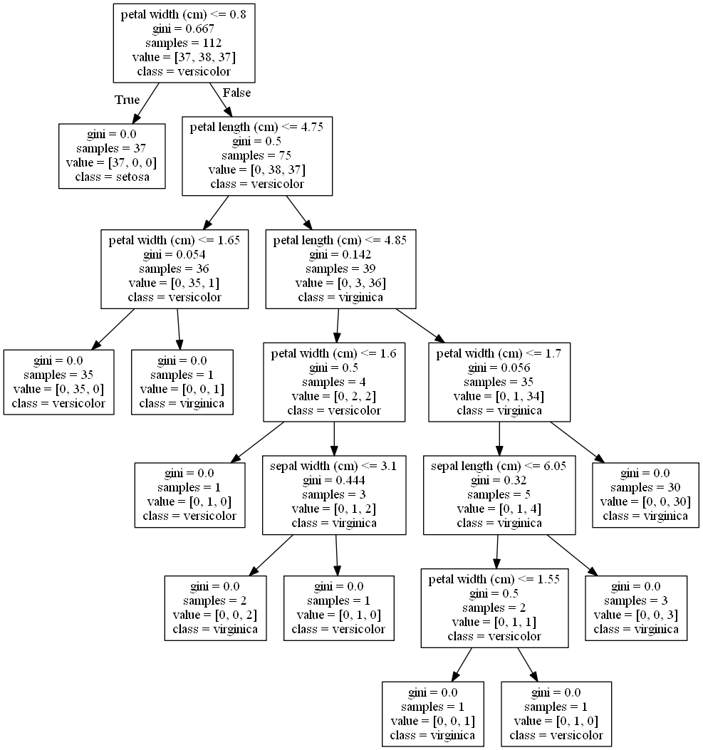
# 참고: https://www.kaggle.com/vaishvik25/titanic-eda-fe-3-model-decision-tree-viz from sklearn.tree import DecisionTreeClassifier, export_graphviz
tree_dot = export_graphviz(dt,out_file=None, feature_names=feature_names, class_names=np.unique(iris['target_names'])) tree = graphviz.Source(tree_dot) tree
gini계수: 불순도를 의미함. gini계수가 높을 수록 엔트로피(Entropy)가 큼. 즉, 클래스가 혼잡하게 섞여 있음.
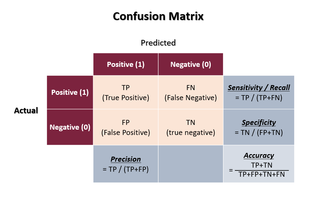
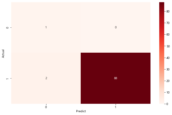
정확도는 모델의 성능을 가장 지관적으로 나타낼 수 있는 평가 지표다. 하지만, 만약 Actual positive sample과 Actual negative sample의 비율이 차이가 많이 나면 정확도의 함정에 빠질 수 있다.
즉, 모두 positive / negative로 예측 했을 때 모델의 정확도가 매우 높은 경우다. 이 경우에 예측 정확도가 높지만, 모델의 예측 성능이 좋다라고 말할 수는 없다.
유방암 환자 데이터셋을 이용하여 한번 이해해 볼게요.
1 2 3
from sklearn.datasets import load_breast_cancer from sklearn.model_selection import train_test_split import numpy as np
1
cancer = load_breast_cancer(유방암 환자 데이터셋)
1
print(cancer['DESCR']) # describe
.. _breast_cancer_dataset:
Breast cancer wisconsin (diagnostic) dataset
--------------------------------------------
**Data Set Characteristics:**
:Number of Instances: 569
:Number of Attributes: 30 numeric, predictive attributes and the class
:Attribute Information:
- radius (mean of distances from center to points on the perimeter)
- texture (standard deviation of gray-scale values)
- perimeter
- area
- smoothness (local variation in radius lengths)
- compactness (perimeter^2 / area - 1.0)
- concavity (severity of concave portions of the contour)
- concave points (number of concave portions of the contour)
- symmetry
- fractal dimension ("coastline approximation" - 1)
The mean, standard error, and "worst" or largest (mean of the three
largest values) of these features were computed for each image,
resulting in 30 features. For instance, field 3 is Mean Radius, field
13 is Radius SE, field 23 is Worst Radius.
- class:
- WDBC-Malignant
- WDBC-Benign
:Summary Statistics:
===================================== ====== ======
Min Max
===================================== ====== ======
radius (mean): 6.981 28.11
texture (mean): 9.71 39.28
perimeter (mean): 43.79 188.5
area (mean): 143.5 2501.0
smoothness (mean): 0.053 0.163
compactness (mean): 0.019 0.345
concavity (mean): 0.0 0.427
concave points (mean): 0.0 0.201
symmetry (mean): 0.106 0.304
fractal dimension (mean): 0.05 0.097
radius (standard error): 0.112 2.873
texture (standard error): 0.36 4.885
perimeter (standard error): 0.757 21.98
area (standard error): 6.802 542.2
smoothness (standard error): 0.002 0.031
compactness (standard error): 0.002 0.135
concavity (standard error): 0.0 0.396
concave points (standard error): 0.0 0.053
symmetry (standard error): 0.008 0.079
fractal dimension (standard error): 0.001 0.03
radius (worst): 7.93 36.04
texture (worst): 12.02 49.54
perimeter (worst): 50.41 251.2
area (worst): 185.2 4254.0
smoothness (worst): 0.071 0.223
compactness (worst): 0.027 1.058
concavity (worst): 0.0 1.252
concave points (worst): 0.0 0.291
symmetry (worst): 0.156 0.664
fractal dimension (worst): 0.055 0.208
===================================== ====== ======
:Missing Attribute Values: None
:Class Distribution: 212 - Malignant, 357 - Benign
:Creator: Dr. William H. Wolberg, W. Nick Street, Olvi L. Mangasarian
:Donor: Nick Street
:Date: November, 1995
This is a copy of UCI ML Breast Cancer Wisconsin (Diagnostic) datasets.
https://goo.gl/U2Uwz2
Features are computed from a digitized image of a fine needle
aspirate (FNA) of a breast mass. They describe
characteristics of the cell nuclei present in the image.
Separating plane described above was obtained using
Multisurface Method-Tree (MSM-T) [K. P. Bennett, "Decision Tree
Construction Via Linear Programming." Proceedings of the 4th
Midwest Artificial Intelligence and Cognitive Science Society,
pp. 97-101, 1992], a classification method which uses linear
programming to construct a decision tree. Relevant features
were selected using an exhaustive search in the space of 1-4
features and 1-3 separating planes.
The actual linear program used to obtain the separating plane
in the 3-dimensional space is that described in:
[K. P. Bennett and O. L. Mangasarian: "Robust Linear
Programming Discrimination of Two Linearly Inseparable Sets",
Optimization Methods and Software 1, 1992, 23-34].
This database is also available through the UW CS ftp server:
ftp ftp.cs.wisc.edu
cd math-prog/cpo-dataset/machine-learn/WDBC/
.. topic:: References
- W.N. Street, W.H. Wolberg and O.L. Mangasarian. Nuclear feature extraction
for breast tumor diagnosis. IS&T/SPIE 1993 International Symposium on
Electronic Imaging: Science and Technology, volume 1905, pages 861-870,
San Jose, CA, 1993.
- O.L. Mangasarian, W.N. Street and W.H. Wolberg. Breast cancer diagnosis and
prognosis via linear programming. Operations Research, 43(4), pages 570-577,
July-August 1995.
- W.H. Wolberg, W.N. Street, and O.L. Mangasarian. Machine learning techniques
to diagnose breast cancer from fine-needle aspirates. Cancer Letters 77 (1994)
163-171.
1 2 3
data = cancer['data'] target = cancer['target'] feature_names = cancer['feature_names']
1
2
3
# 데이터 프레임 생성
df = pd.DataFrame(data = data, columns = feature_names)
df['target'] = target