0. 개요 포켓몬 데이터셋을 이용해 분류 분석을 진행합니다.
지도 학습 (Logistic Regression): “전설의 포켓몬” 여부 예측 – “Legendary” = 0/1비지도 학습 (K-Means Clustering): 포켓몬 군집 분석
1. Library & Data Import >> 사용할 Library
1
2
3
4
5
6
7
8
9
%matplotlib inline import pandas as pdimport numpy as npimport matplotlib.pyplot as pltimport seaborn as snsimport warningswarnings.filterwarnings("ignore" )
1 plt.rcParams['font.family' ] = 'Malgun Gothic'
1 plt.rcParams['figure.figsize' ] = (10 , 8 )
>> 사용할 데이터셋 - Pokemon Dataset
1 df = pd.read_csv("https://raw.githubusercontent.com/yoonkt200/FastCampusDataset/master/Pokemon.csv" )
#
Name
Type 1
Type 2
Total
HP
Attack
Defense
Sp. Atk
Sp. Def
Speed
Generation
Legendary
0
1
Bulbasaur
Grass
Poison
318
45
49
49
65
65
45
1
False
1
2
Ivysaur
Grass
Poison
405
60
62
63
80
80
60
1
False
2
3
Venusaur
Grass
Poison
525
80
82
83
100
100
80
1
False
3
3
VenusaurMega Venusaur
Grass
Poison
625
80
100
123
122
120
80
1
False
4
4
Charmander
Fire
NaN
309
39
52
43
60
50
65
1
False
>> Feature Description
Name: 포켓몬 이름
Type 1: 포켓몬 타입 1
Type 2: 포켓몬 타입 2
Total: 포켓몬 총 능력치 (Sum of ‘HP’, ‘Attack’, ‘Defense’, ‘Sp.Atk’, ‘Sp.Def’ and ‘Speed’)
HP: 포켓몬 HP 능력치
Attack: 포켓몬 Attack 능력치
Defense: 포켓몬 Defense 능력치
Sp.Atk: 포켓몬 Sp.Atk 능력치
Sp.Def: 포켓몬 Sp.Def 능력치
Speed: 포켓몬 Speed 능력치
Generation: 포켓몬 세대
Legendary: 전설의 포켓몬 여부
2. EDA (Exploratoty Data Analysis: 탐색적 데이터 분석) 1 2 sns.set_style('darkgrid' )
>> 전체 데이터셋
(800, 13)
<class 'pandas.core.frame.DataFrame'>
RangeIndex: 800 entries, 0 to 799
Data columns (total 13 columns):
# Column Non-Null Count Dtype
--- ------ -------------- -----
0 # 800 non-null int64
1 Name 800 non-null object
2 Type 1 800 non-null object
3 Type 2 414 non-null object
4 Total 800 non-null int64
5 HP 800 non-null int64
6 Attack 800 non-null int64
7 Defense 800 non-null int64
8 Sp. Atk 800 non-null int64
9 Sp. Def 800 non-null int64
10 Speed 800 non-null int64
11 Generation 800 non-null int64
12 Legendary 800 non-null bool
dtypes: bool(1), int64(9), object(3)
memory usage: 75.9+ KB
# 0
Name 0
Type 1 0
Type 2 386
Total 0
HP 0
Attack 0
Defense 0
Sp. Atk 0
Sp. Def 0
Speed 0
Generation 0
Legendary 0
dtype: int64
>> 개별 Feature 탐색
분류할 목표 Feature : “Legendary” (전설의 포켓몬 여부)
1 2 df['Legendary' ].value_counts()
False 735
True 65
Name: Legendary, dtype: int64
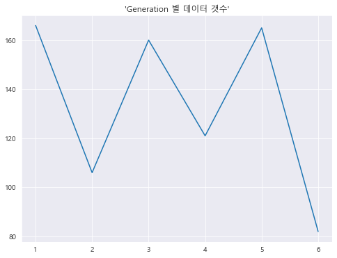
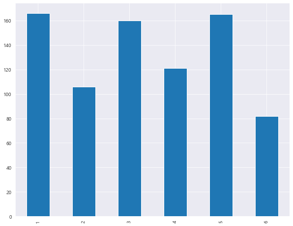
1 2 df['Generation' ].value_counts()
1 166
5 165
3 160
4 121
2 106
6 82
Name: Generation, dtype: int64
1 2 3 4 5 fig = plt.figure(figsize=(8 , 6 )) df['Generation' ].value_counts().sort_index().plot() plt.title("'Generation 별 데이터 갯수'" ) plt.show()
“Type 1” & “Type 2” (포켓몬 타입)
array(['Grass', 'Fire', 'Water', 'Bug', 'Normal', 'Poison', 'Electric',
'Ground', 'Fairy', 'Fighting', 'Psychic', 'Rock', 'Ghost', 'Ice',
'Dragon', 'Dark', 'Steel', 'Flying'], dtype=object)
1 2 len(df['Type 1' ].unique())
18
1 2 df[df['Type 2' ].notnull()]['Type 2' ].unique()
array(['Poison', 'Flying', 'Dragon', 'Ground', 'Fairy', 'Grass',
'Fighting', 'Psychic', 'Steel', 'Ice', 'Rock', 'Dark', 'Water',
'Electric', 'Fire', 'Ghost', 'Bug', 'Normal'], dtype=object)
1 2 len(df[df['Type 2' ].notnull()]['Type 2' ].unique())
18
각 변수(Feature)의 분포를 관찰함으로써, 변수들의 특징을 알아보도록 하겠습니다.
특히, 저희가 분류할 목표 Feature가 "Legendary"이므로, 각 변수의 분포를 탐색 시:
각 항목(feature)에서 전체 데이터의 분포 뿐만 아닌
"Legendary"변수 class 별의 데이터 분포 도 함께 살펴볼게요.
GUIDE
【전체 데이터 탐색】 & 【“Legendary” class별 탐색】
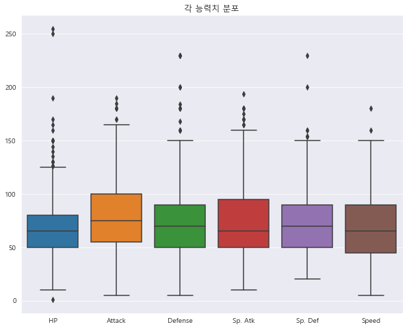
각 능력치 분포
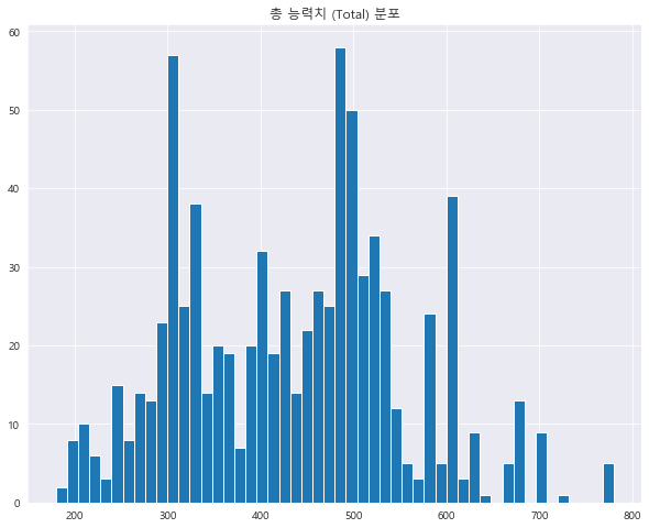
총 능력치 (Toal) 분포
포켓몬 타입 (Type 1 & Type 2) 분포
포켓몬 세대 (Generation) 분포
1 2 3 4 5 6 stats = ['HP' , 'Attack' , 'Defense' , 'Sp. Atk' , 'Sp. Def' , 'Speed' ] sns.boxplot(data = df[stats]) plt.title('각 능력치 분포' ) plt.show()
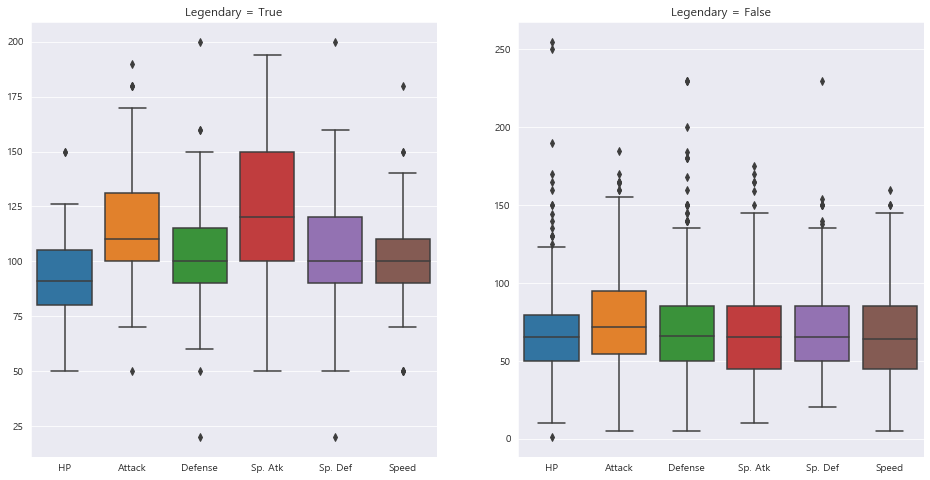
1 2 3 4 5 6 7 8 9 10 11 12 13 fig = plt.figure(figsize=(16 , 8 )) plt.subplot(1 ,2 ,1 ) sns.boxplot(data = df[df['Legendary' ]==1 ][stats]) plt.title('Legendary = True' ) plt.subplot(1 ,2 ,2 ) sns.boxplot(data = df[df['Legendary' ]==0 ][stats]) plt.title('Legendary = False' ) plt.show()
"전설의 포켓몬"은 전체적으로 더 높은 능력치를 보유하고 있으며, Attack와 Sp.Atk가 특히 높은 것으로 보입니다.
1 2 3 4 5 df['Total' ].hist(bins=50 ) plt.title('총 능력치 (Total) 분포' ) plt.show()
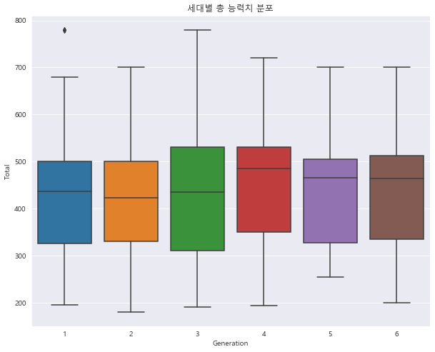
1 2 3 4 sns.boxplot(data = df, x = "Generation" , y="Total" ) plt.title("세대별 총 능력치 분포" ) plt.show()
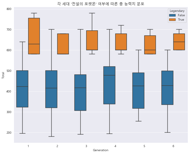
1 2 3 4 sns.boxplot(data = df, x = "Generation" , y="Total" , hue="Legendary" ) plt.title("각 세대 '전설의 포켓몬' 여부에 따른 총 능력치 분포" ) plt.show()
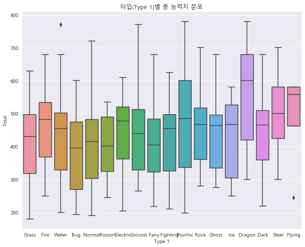
1 2 3 4 sns.boxplot(data = df, x = 'Type 1' , y = 'Total' ) plt.title("타입(Type 1)별 총 능력치 분포" ) plt.show()
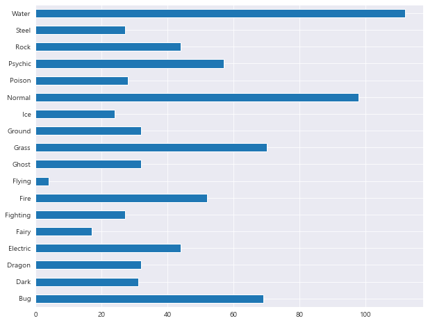
1 2 3 df['Type 1' ].value_counts(sort=False ).sort_index().plot.barh()
<matplotlib.axes._subplots.AxesSubplot at 0x2e92fab51c8>
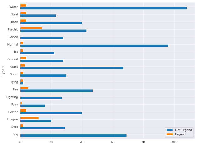
1 2 3 4 5 6 7 8 T1_Total = pd.DataFrame(df['Type 1' ].value_counts().sort_index()) T1_NotLeg = pd.DataFrame(df[df['Legendary' ]==0 ].groupby('Type 1' ).size()) T1_count = pd.concat([T1_Total, T1_NotLeg], axis = 1 ) T1_count.columns = ['Total' , 'Not Legend' ] T1_count['Legend' ] = T1_count['Total' ] - T1_count['Not Legend' ] T1_count
Total
Not Legend
Legend
Type 1
Bug
69
69
0
Dark
31
29
2
Dragon
32
20
12
Electric
44
40
4
Fairy
17
16
1
Fighting
27
27
0
Fire
52
47
5
Flying
4
2
2
Ghost
32
30
2
Grass
70
67
3
Ground
32
28
4
Ice
24
22
2
Normal
98
96
2
Poison
28
28
0
Psychic
57
43
14
Rock
44
40
4
Steel
27
23
4
Water
112
108
4
1 T1_count[['Not Legend' , 'Legend' ]].plot.barh(width=0.7 )
<matplotlib.axes._subplots.AxesSubplot at 0x2e92ff18b88>
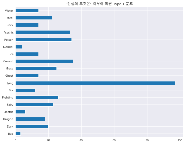
1 2 3 4 5 6 df['Type 2' ].value_counts(sort=False ).sort_index().plot.barh() plt.title('"전설의 포켓몬" 여부에 따른 Type 1 분포' ) plt.show()
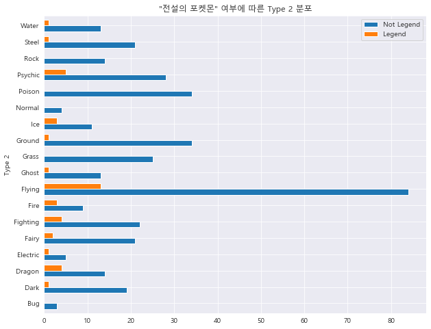
1 2 3 4 5 6 7 8 T2_Total = pd.DataFrame(df['Type 2' ].value_counts().sort_index()) T2_NotLeg = pd.DataFrame(df[df['Legendary' ]==0 ].groupby('Type 2' ).size()) T2_count = pd.concat([T2_Total, T2_NotLeg], axis = 1 ) T2_count.columns = ['Total' , 'Not Legend' ] T2_count['Legend' ] = T2_count['Total' ] - T2_count['Not Legend' ] T2_count
Total
Not Legend
Legend
Type 2
Bug
3
3
0
Dark
20
19
1
Dragon
18
14
4
Electric
6
5
1
Fairy
23
21
2
Fighting
26
22
4
Fire
12
9
3
Flying
97
84
13
Ghost
14
13
1
Grass
25
25
0
Ground
35
34
1
Ice
14
11
3
Normal
4
4
0
Poison
34
34
0
Psychic
33
28
5
Rock
14
14
0
Steel
22
21
1
Water
14
13
1
1 2 3 4 T2_count[['Not Legend' , 'Legend' ]].plot.barh(width=0.7 ) plt.title('"전설의 포켓몬" 여부에 따른 Type 2 분포' ) plt.show()
1 2 3 df['Generation' ].value_counts().sort_index().plot.bar()
<matplotlib.axes._subplots.AxesSubplot at 0x2e930887d08>
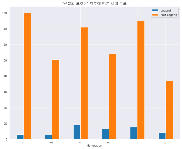
1 2 3 4 5 6 7 gene_Leg = pd.DataFrame(df[df['Legendary' ]==1 ].groupby('Generation' ).size()) gene_NotLeg = pd.DataFrame(df[df['Legendary' ]==0 ].groupby('Generation' ).size()) gene_count = pd.concat([gene_Leg, gene_NotLeg], axis=1 ) gene_count.columns = ['Legend' , 'Not Legend' ] gene_count
Legend
Not Legend
Generation
1
6
160
2
5
101
3
18
142
4
13
108
5
15
150
6
8
74
1 2 3 gene_count.plot.bar() plt.title('"전설의 포켓몬" 여부에 따른 세대 분포' ) plt.show()
3. 지도 학습 기반 분류 분석 – Logistic Regression
#
Name
Type 1
Type 2
Total
HP
Attack
Defense
Sp. Atk
Sp. Def
Speed
Generation
Legendary
0
1
Bulbasaur
Grass
Poison
318
45
49
49
65
65
45
1
False
1
2
Ivysaur
Grass
Poison
405
60
62
63
80
80
60
1
False
2
3
Venusaur
Grass
Poison
525
80
82
83
100
100
80
1
False
3
3
VenusaurMega Venusaur
Grass
Poison
625
80
100
123
122
120
80
1
False
4
4
Charmander
Fire
NaN
309
39
52
43
60
50
65
1
False
<class 'pandas.core.frame.DataFrame'>
RangeIndex: 800 entries, 0 to 799
Data columns (total 13 columns):
 #   Column      Non-Null Count  Dtype
---  ------      --------------  -----
 0   #           800 non-null    int64
 1   Name        800 non-null    object
 2   Type 1      800 non-null    object
 3   Type 2      414 non-null    object
 4   Total       800 non-null    int64
 5   HP          800 non-null    int64
 6   Attack      800 non-null    int64
 7   Defense     800 non-null    int64
 8   Sp. Atk     800 non-null    int64
 9   Sp. Def     800 non-null    int64
 10  Speed       800 non-null    int64
 11  Generation  800 non-null    int64
 12  Legendary   800 non-null    bool
dtypes: bool(1), int64(9), object(3)
memory usage: 75.9+ KB
분류예측 목표 Feature인 "Lengendary"의 값은 현재 “True”/"False"로 구성되어있습니다. 예측 모델에 적용하기 위해 “1”/"0"으로 바꾸겠습니다.
포켓몬의 세대를 나타나는 Feature인 "Generation"의 타입은 지금 "int"로 되어있지만, Feature의 의미상 해당 숫자는 분류 역할을 하고 있으므로 "str"타입으로 변환시키겠습니다.
분류 예측 시 이름 데이터가 예측에 도움이 없으므로 "Name"을 빼고 데이터셋을 제구성하겠습니다.
1 2 3 4 5 df['Legendary' ] = df['Legendary' ].astype(int) df['Generation' ] = df['Generation' ].astype(str) preprocessed_df = df[['Type 1' , 'Type 2' , 'Total' , 'HP' , 'Attack' , 'Defense' , 'Sp. Atk' , 'Sp. Def' , 'Speed' , 'Generation' , 'Legendary' ]] preprocessed_df.head()
Type 1
Type 2
Total
HP
Attack
Defense
Sp. Atk
Sp. Def
Speed
Generation
Legendary
0
Grass
Poison
318
45
49
49
65
65
45
1
0
1
Grass
Poison
405
60
62
63
80
80
60
1
0
2
Grass
Poison
525
80
82
83
100
100
80
1
0
3
Grass
Poison
625
80
100
123
122
120
80
1
0
4
Fire
NaN
309
39
52
43
60
50
65
1
0
Categorical Variable에 대해서 dummy화 작업을 진행하겠습니다.
>> 타입 (Type) – Multi-label Encoding
먼저 Type 1과 Type 2를 하나의 변수(Type)로 묶는다.
그 다음 1~2개의 label를 가진 Type변수에 대해서 Multi-label Encoding을 진행한다.
1 2 3 4 5 6 7 8 9 10 def make_list (x1, x2) : type_list = [] type_list.append(x1) if x2 is not np.nan: type_list.append(x2) return type_list preprocessed_df['Type' ] = preprocessed_df.apply(lambda x: make_list(x['Type 1' ], x['Type 2' ]), axis=1 ) preprocessed_df.head()
Type 1
Type 2
Total
HP
Attack
Defense
Sp. Atk
Sp. Def
Speed
Generation
Legendary
Type
0
Grass
Poison
318
45
49
49
65
65
45
1
0
[Grass, Poison]
1
Grass
Poison
405
60
62
63
80
80
60
1
0
[Grass, Poison]
2
Grass
Poison
525
80
82
83
100
100
80
1
0
[Grass, Poison]
3
Grass
Poison
625
80
100
123
122
120
80
1
0
[Grass, Poison]
4
Fire
NaN
309
39
52
43
60
50
65
1
0
[Fire]
1 2 3 del preprocessed_df['Type 1' ]del preprocessed_df['Type 2' ]preprocessed_df.head()
Total
HP
Attack
Defense
Sp. Atk
Sp. Def
Speed
Generation
Legendary
Type
0
318
45
49
49
65
65
45
1
0
[Grass, Poison]
1
405
60
62
63
80
80
60
1
0
[Grass, Poison]
2
525
80
82
83
100
100
80
1
0
[Grass, Poison]
3
625
80
100
123
122
120
80
1
0
[Grass, Poison]
4
309
39
52
43
60
50
65
1
0
[Fire]
1 2 3 4 5 6 from sklearn.preprocessing import MultiLabelBinarizerml = MultiLabelBinarizer() preprocessed_df = preprocessed_df.join(pd.DataFrame(ml.fit_transform(preprocessed_df.pop('Type' )), columns = ml.classes_))
Total
HP
Attack
Defense
Sp. Atk
Sp. Def
Speed
Generation
Legendary
Bug
...
Ghost
Grass
Ground
Ice
Normal
Poison
Psychic
Rock
Steel
Water
0
318
45
49
49
65
65
45
1
0
0
...
0
1
0
0
0
1
0
0
0
0
1
405
60
62
63
80
80
60
1
0
0
...
0
1
0
0
0
1
0
0
0
0
2
525
80
82
83
100
100
80
1
0
0
...
0
1
0
0
0
1
0
0
0
0
3
625
80
100
123
122
120
80
1
0
0
...
0
1
0
0
0
1
0
0
0
0
4
309
39
52
43
60
50
65
1
0
0
...
0
0
0
0
0
0
0
0
0
0
5 rows × 27 columns
>> 세대 (Generation) – One-hot Encoding
1 2 3 4 preprocessed_df = pd.get_dummies(preprocessed_df) preprocessed_df.head()
Total
HP
Attack
Defense
Sp. Atk
Sp. Def
Speed
Legendary
Bug
Dark
...
Psychic
Rock
Steel
Water
Generation_1
Generation_2
Generation_3
Generation_4
Generation_5
Generation_6
0
318
45
49
49
65
65
45
0
0
0
...
0
0
0
0
1
0
0
0
0
0
1
405
60
62
63
80
80
60
0
0
0
...
0
0
0
0
1
0
0
0
0
0
2
525
80
82
83
100
100
80
0
0
0
...
0
0
0
0
1
0
0
0
0
0
3
625
80
100
123
122
120
80
0
0
0
...
0
0
0
0
1
0
0
0
0
0
4
309
39
52
43
60
50
65
0
0
0
...
0
0
0
0
1
0
0
0
0
0
5 rows × 32 columns
Numerical Feature간의 Scale차이를 없애기 위해 feature 표준화를 진행합니다.
<class 'pandas.core.frame.DataFrame'>
RangeIndex: 800 entries, 0 to 799
Data columns (total 32 columns):
# Column Non-Null Count Dtype
--- ------ -------------- -----
0 Total 800 non-null int64
1 HP 800 non-null int64
2 Attack 800 non-null int64
3 Defense 800 non-null int64
4 Sp. Atk 800 non-null int64
5 Sp. Def 800 non-null int64
6 Speed 800 non-null int64
7 Legendary 800 non-null int32
8 Bug 800 non-null int32
9 Dark 800 non-null int32
10 Dragon 800 non-null int32
11 Electric 800 non-null int32
12 Fairy 800 non-null int32
13 Fighting 800 non-null int32
14 Fire 800 non-null int32
15 Flying 800 non-null int32
16 Ghost 800 non-null int32
17 Grass 800 non-null int32
18 Ground 800 non-null int32
19 Ice 800 non-null int32
20 Normal 800 non-null int32
21 Poison 800 non-null int32
22 Psychic 800 non-null int32
23 Rock 800 non-null int32
24 Steel 800 non-null int32
25 Water 800 non-null int32
26 Generation_1 800 non-null uint8
27 Generation_2 800 non-null uint8
28 Generation_3 800 non-null uint8
29 Generation_4 800 non-null uint8
30 Generation_5 800 non-null uint8
31 Generation_6 800 non-null uint8
dtypes: int32(19), int64(7), uint8(6)
memory usage: 107.9 KB
1 2 3 4 5 6 7 from sklearn.preprocessing import StandardScalerscaler = StandardScaler() scale_columns = ['Total' , 'HP' , 'Attack' , 'Defense' , 'Sp. Atk' , 'Sp. Def' , 'Speed' ] preprocessed_df[scale_columns] = scaler.fit_transform(preprocessed_df[scale_columns]) preprocessed_df.head()
Total
HP
Attack
Defense
Sp. Atk
Sp. Def
Speed
Legendary
Bug
Dark
...
Psychic
Rock
Steel
Water
Generation_1
Generation_2
Generation_3
Generation_4
Generation_5
Generation_6
0
-0.976765
-0.950626
-0.924906
-0.797154
-0.239130
-0.248189
-0.801503
0
0
0
...
0
0
0
0
1
0
0
0
0
0
1
-0.251088
-0.362822
-0.524130
-0.347917
0.219560
0.291156
-0.285015
0
0
0
...
0
0
0
0
1
0
0
0
0
0
2
0.749845
0.420917
0.092448
0.293849
0.831146
1.010283
0.403635
0
0
0
...
0
0
0
0
1
0
0
0
0
0
3
1.583957
0.420917
0.647369
1.577381
1.503891
1.729409
0.403635
0
0
0
...
0
0
0
0
1
0
0
0
0
0
4
-1.051836
-1.185748
-0.832419
-0.989683
-0.392027
-0.787533
-0.112853
0
0
0
...
0
0
0
0
1
0
0
0
0
0
5 rows × 32 columns
1 2 3 4 5 from sklearn.model_selection import train_test_splitX = preprocessed_df.loc[:, preprocessed_df.columns != 'Legendary' ] y = preprocessed_df['Legendary' ] x_train, x_test, y_train, y_test = train_test_split(X, y, test_size=0.25 , random_state=1 )
1 x_train.shape, y_train.shape
((600, 31), (600,))
1 x_test.shape, y_test.shape
((200, 31), (200,))
1 2 3 4 5 6 7 8 9 from sklearn.linear_model import LogisticRegressionfrom sklearn.metrics import accuracy_score, precision_score, recall_score, f1_scorelogit = LogisticRegression(random_state=0 ) logit.fit(x_train, y_train) y_pred = logit.predict(x_test)
1 2 3 4 5 6 print("accuracy: %.2f" % accuracy_score(y_test, y_pred)) print("Precision: %.3f" % precision_score(y_test, y_pred)) print("Recall: %.3f" % recall_score(y_test, y_pred)) print("F1: %.3f" % f1_score(y_test, y_pred))
accuracy: 0.93
Precision: 0.615
Recall: 0.471
F1: 0.533
위 모델 평가 결과를 확인해보면, 해당 모델은 정확도(accuracy) 만 높고, 정밀도(Precision), 재현율(Recall), F1 score 등 모두 낮습니다. 이는 학습 데이터의 클래스 불균형으로 인한 정확도 함정 문제일 가능성이 높습니다. (참고: [Python >> sklearn - (2) 분류] 4-2. !!정확도 함정!! )
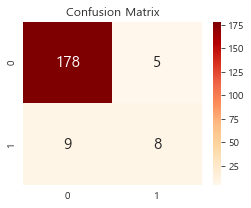
추가 확인을 위해 Confusion Matrix를 출력해 봅니다.
1 np.set_printoptions(suppress=True )
1 2 3 4 5 6 7 8 9 from sklearn.metrics import confusion_matrixconfu = confusion_matrix(y_true = y_test, y_pred = y_pred) plt.figure(figsize=(4 , 3 )) sns.heatmap(confu, annot=True , annot_kws={'size' :15 }, cmap='OrRd' , fmt='.10g' ) plt.title('Confusion Matrix' ) plt.show()
Positive Condition ( “Legendary” = True/1 ) <17> 대비 Negative Condition ( “Legendary” = False/0 ) <183>인 케이스가 훨씬 많다는 것을 볼 수 있습니다. 따라서, 클래스 불균형으로 인한 정확도 함정 문제가 맞으며, 클래스 불균형을 조정 한 후 다시 학습 시키도록 하겠습니다.
1 preprocessed_df['Legendary' ].value_counts()
0 735
1 65
Name: Legendary, dtype: int64
>> 1:1 샘플링
Positive Condition 케이스와 Negative Condition 케이스를 1:1비율로 샘플링 합니다.
1 2 positive_random_idx = preprocessed_df[preprocessed_df['Legendary' ]==1 ].sample(65 , random_state=12 ).index.tolist() negative_random_idx = preprocessed_df[preprocessed_df['Legendary' ]==0 ].sample(65 , random_state=12 ).index.tolist()
>> Training set / Test set 나누기
1 2 3 4 random_idx = positive_random_idx + negative_random_idx X = preprocessed_df.loc[random_idx, preprocessed_df.columns != 'Legendary' ] y = preprocessed_df['Legendary' ][random_idx] x_train, x_test, y_train, y_test = train_test_split(X, y, test_size=0.25 , random_state=1 )
1 x_train.shape, y_train.shape
((97, 31), (97,))
1 x_test.shape, y_test.shape
((33, 31), (33,))
>> 모델 재학습
1 2 3 4 5 6 logit2 = LogisticRegression(random_state=0 ) logit2.fit(x_train, y_train) y_pred2 = logit2.predict(x_test)
>> 모델 재평가
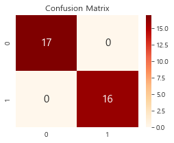
1 2 3 4 5 6 print("accuracy: %.2f" % accuracy_score(y_test, y_pred2)) print("Precision: %.3f" % precision_score(y_test, y_pred2)) print("Recall: %.3f" % recall_score(y_test, y_pred2)) print("F1: %.3f" % f1_score(y_test, y_pred2))
accuracy: 1.00
Precision: 1.000
Recall: 1.000
F1: 1.000
1 2 3 4 5 6 7 8 confu2 = confusion_matrix(y_true=y_test, y_pred = y_pred2) plt.figure(figsize=(4 , 3 )) sns.heatmap(confu2, annot=True , annot_kws={'size' :15 }, cmap='OrRd' , fmt='.10g' ) plt.title('Confusion Matrix' ) plt.show()
클래스 불균형을 조정한 후, 새롭게 학습된 모델의 performance가 많이 좋아졌습니다.
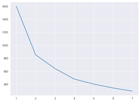
4. 비지도 학습 기반 군집 분석 – K-Means Clustering 1 2 3 4 5 6 7 8 9 10 11 12 13 14 15 16 from sklearn.cluster import KMeansX = preprocessed_df[['Attack' , 'Defense' ]] k_list = [] cost_list = [] for k in range (1 , 8 ): kmeans = KMeans(n_clusters=k).fit(X) interia = kmeans.inertia_ print("k:" , k, "| cost:" , interia) k_list.append(k) cost_list.append(interia) plt.figure(figsize=(8 , 6 )) plt.plot(k_list, cost_list)
k: 1 | cost: 1600.0
k: 2 | cost: 853.3477298974242
k: 3 | cost: 642.3911470107209
k: 4 | cost: 480.49450250321513
k: 5 | cost: 403.97191765107124
k: 6 | cost: 343.98696660525184
k: 7 | cost: 295.56093457429847
[<matplotlib.lines.Line2D at 0x2e930467c48>]
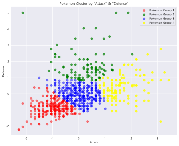
추세를 봤을 때, 4 clusters가 제일 적당한 것으로 보입니다.
따라서, cluster를 4로 지정한 후 다시 학습시킨 뒤, 각 데이터가 분류된 cluster 결과를 원 데이터셋에 추가합니다.
1 2 3 4 5 kmeans = KMeans(n_clusters=4 ).fit(X) cluster_num = pd.Series(kmeans.predict(X)) preprocessed_df['cluster_num' ] = cluster_num.values preprocessed_df.head()
Total
HP
Attack
Defense
Sp. Atk
Sp. Def
Speed
Legendary
Bug
Dark
...
Rock
Steel
Water
Generation_1
Generation_2
Generation_3
Generation_4
Generation_5
Generation_6
cluster_num
0
-0.976765
-0.950626
-0.924906
-0.797154
-0.239130
-0.248189
-0.801503
0
0
0
...
0
0
0
1
0
0
0
0
0
0
1
-0.251088
-0.362822
-0.524130
-0.347917
0.219560
0.291156
-0.285015
0
0
0
...
0
0
0
1
0
0
0
0
0
2
2
0.749845
0.420917
0.092448
0.293849
0.831146
1.010283
0.403635
0
0
0
...
0
0
0
1
0
0
0
0
0
2
3
1.583957
0.420917
0.647369
1.577381
1.503891
1.729409
0.403635
0
0
0
...
0
0
0
1
0
0
0
0
0
1
4
-1.051836
-1.185748
-0.832419
-0.989683
-0.392027
-0.787533
-0.112853
0
0
0
...
0
0
0
1
0
0
0
0
0
0
5 rows × 33 columns
1 print(preprocessed_df['cluster_num' ].value_counts())
2 309
0 253
3 128
1 110
Name: cluster_num, dtype: int64
>> 군집 시각화
1 2 3 4 5 6 7 8 9 10 11 12 13 14 15 16 17 18 19 20 plt.scatter(preprocessed_df[preprocessed_df['cluster_num' ] == 0 ]['Attack' ], preprocessed_df[preprocessed_df['cluster_num' ] == 0 ]['Defense' ], s = 50 , c = 'red' , alpha = 0.5 , label = 'Pokemon Group 1' ) plt.scatter(preprocessed_df[preprocessed_df['cluster_num' ] == 1 ]['Attack' ], preprocessed_df[preprocessed_df['cluster_num' ] == 1 ]['Defense' ], s = 50 , c = 'green' , alpha = 0.7 , label = 'Pokemon Group 2' ) plt.scatter(preprocessed_df[preprocessed_df['cluster_num' ] == 2 ]['Attack' ], preprocessed_df[preprocessed_df['cluster_num' ] == 2 ]['Defense' ], s = 50 , c = 'blue' , alpha = 0.5 , label = 'Pokemon Group 3' ) plt.scatter(preprocessed_df[preprocessed_df['cluster_num' ] == 3 ]['Attack' ], preprocessed_df[preprocessed_df['cluster_num' ] == 3 ]['Defense' ], s = 50 , c = 'yellow' , alpha = 0.8 , label = 'Pokemon Group 4' ) plt.title('Pokemon Cluster by "Attack" & "Defense"' ) plt.xlabel('Attack' ) plt.ylabel('Defense' ) plt.legend() plt.show()
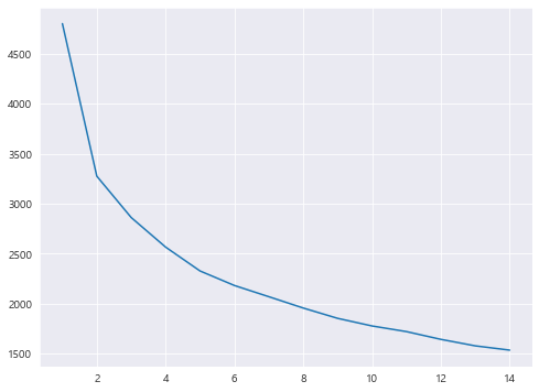
1 2 3 4 5 6 7 8 9 10 11 12 13 14 15 16 from sklearn.cluster import KMeansX = preprocessed_df[['HP' , 'Attack' , 'Defense' , 'Sp. Atk' , 'Sp. Def' , 'Speed' ]] k_list = [] cost_list = [] for k in range (1 , 15 ): kmeans = KMeans(n_clusters=k).fit(X) interia = kmeans.inertia_ print("k:" , k, "| cost:" , interia) k_list.append(k) cost_list.append(interia) plt.figure(figsize=(8 , 6 )) plt.plot(k_list, cost_list)
k: 1 | cost: 4800.0
k: 2 | cost: 3275.3812330305977
k: 3 | cost: 2862.057922495397
k: 4 | cost: 2566.5807792995274
k: 5 | cost: 2328.0706840275643
k: 6 | cost: 2182.759972635841
k: 7 | cost: 2070.734327066247
k: 8 | cost: 1957.5240844927844
k: 9 | cost: 1854.3770148227836
k: 10 | cost: 1778.3178764912984
k: 11 | cost: 1721.845255688537
k: 12 | cost: 1644.3967658442484
k: 13 | cost: 1579.4938049394318
k: 14 | cost: 1536.785887021493
[<matplotlib.lines.Line2D at 0x2e930efbb88>]
이 경우에는 cluster가 5일 때가 제일 적당해 보입니다.
1 2 3 4 5 kmeans = KMeans(n_clusters=5 ).fit(X) cluster_num = pd.Series(kmeans.predict(X)) preprocessed_df['cluster_num' ] = cluster_num.values preprocessed_df.head()
Total
HP
Attack
Defense
Sp. Atk
Sp. Def
Speed
Legendary
Bug
Dark
...
Rock
Steel
Water
Generation_1
Generation_2
Generation_3
Generation_4
Generation_5
Generation_6
cluster_num
0
-0.976765
-0.950626
-0.924906
-0.797154
-0.239130
-0.248189
-0.801503
0
0
0
...
0
0
0
1
0
0
0
0
0
4
1
-0.251088
-0.362822
-0.524130
-0.347917
0.219560
0.291156
-0.285015
0
0
0
...
0
0
0
1
0
0
0
0
0
1
2
0.749845
0.420917
0.092448
0.293849
0.831146
1.010283
0.403635
0
0
0
...
0
0
0
1
0
0
0
0
0
1
3
1.583957
0.420917
0.647369
1.577381
1.503891
1.729409
0.403635
0
0
0
...
0
0
0
1
0
0
0
0
0
0
4
-1.051836
-1.185748
-0.832419
-0.989683
-0.392027
-0.787533
-0.112853
0
0
0
...
0
0
0
1
0
0
0
0
0
4
5 rows × 33 columns
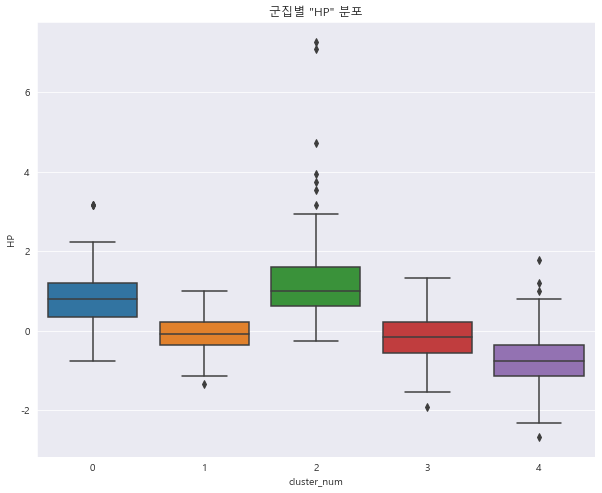
>> 군집별 특성 시각화
2차원이 아니기 때문에 위와 같이 군집 결과를 시각화하기 어렵습니다.
군집화 결과를 확인하기 위해 각 Feature의 군집별 특성 을 시각화하도록 하겠습니다.
1 2 3 4 sns.boxplot(x = "cluster_num" , y = "HP" , data = preprocessed_df) plt.title('군집별 "HP" 분포' ) plt.show()
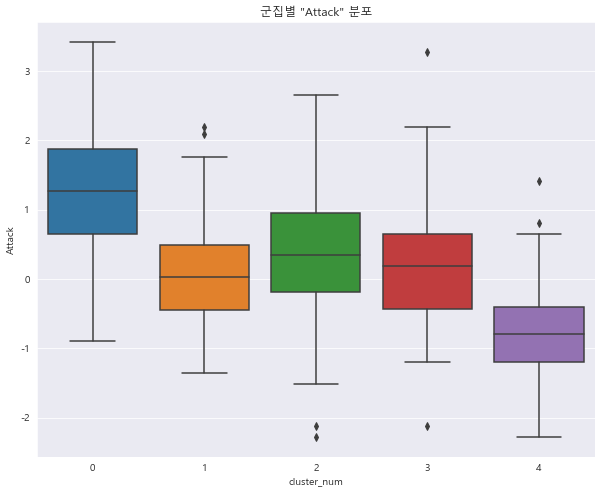
1 2 3 4 sns.boxplot(x = 'cluster_num' , y = 'Attack' , data = preprocessed_df) plt.title('군집별 "Attack" 분포' ) plt.show()
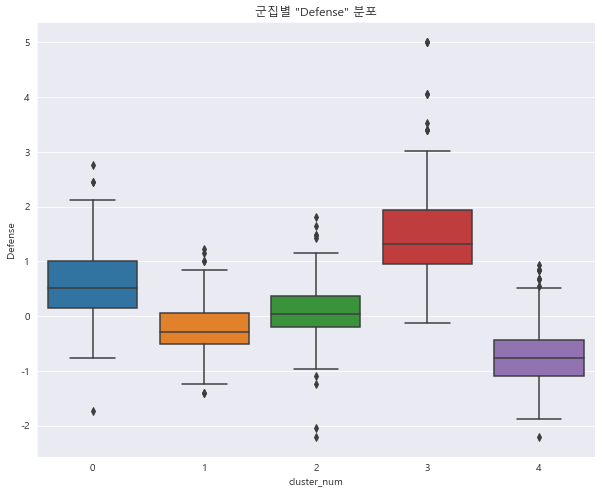
1 2 3 4 sns.boxplot(x = 'cluster_num' , y = 'Defense' , data = preprocessed_df) plt.title('군집별 "Defense" 분포' ) plt.show()
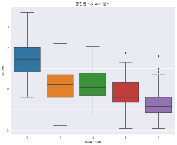
1 2 3 4 sns.boxplot(x = 'cluster_num' , y = 'Sp. Atk' , data = preprocessed_df) plt.title('군집별 "Sp. Atk" 분포' ) plt.show()
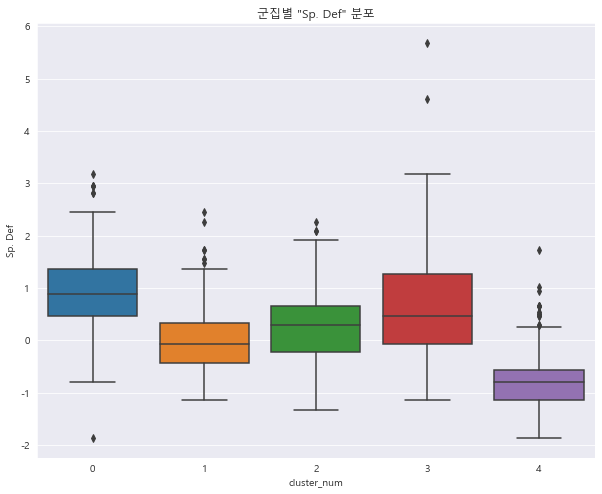
1 2 3 4 sns.boxplot(x = 'cluster_num' , y = 'Sp. Def' , data = preprocessed_df) plt.title('군집별 "Sp. Def" 분포' ) plt.show()
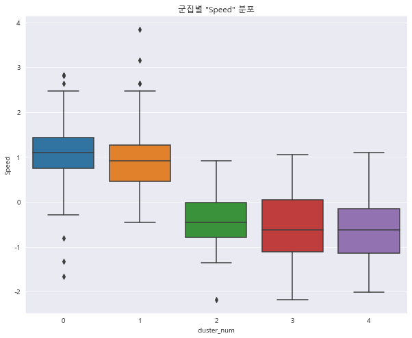
1 2 3 4 sns.boxplot(x = 'cluster_num' , y = 'Speed' , data = preprocessed_df) plt.title('군집별 "Speed" 분포' ) plt.show()