Tableau >> Advanced (5) Geographic Analysis

Geographic Analysis

• 1. Map Dense Data with Hexbins
  • >> Create a hexbin map
• 2. Map Shapes Using Spatial Files
  • >> Use spatial files to map data

1. Map Dense Data with Hexbins

When we want to see a distribution with just one measure, we use bins to create a histogram. However, if we want to show the density of values across two measures, hexbins (also called as density plots) would be a good choice.

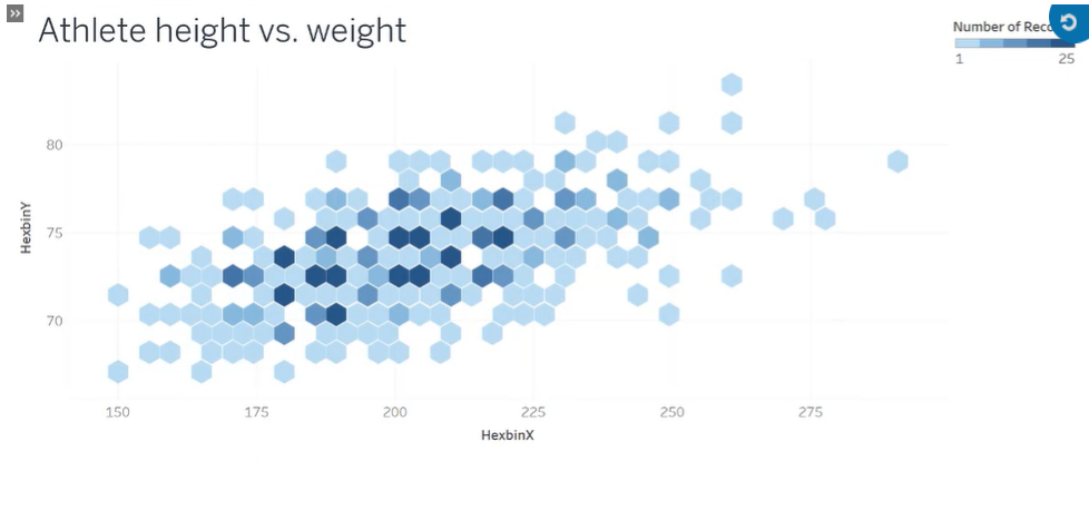
“hexbins” = “hexagons” + "bins"

• "bins" : Much like the bins we create for histograms, hexbins create buckets in the view, which help us to understand the distribution of data.
• "hexagons" : Tessellate – they can cover the view without overlapping or gaps

To create hexbins,

• we use two Tableau built-in calculations: HEXBINX(x, y) & HEXBINY(x, y)

  • HEXBINX assigns values to a bin on the x-axis
  • HEXBINY assigns values to the bin for the y-axis

• and use them both as continuous dimensions:

  • Continuous: let tableau to present an axis, rather than headers
  • Dimensions: let them to behave categorically, rather than aggregate to a sum of HEXBINX, or sum of HEXBINY

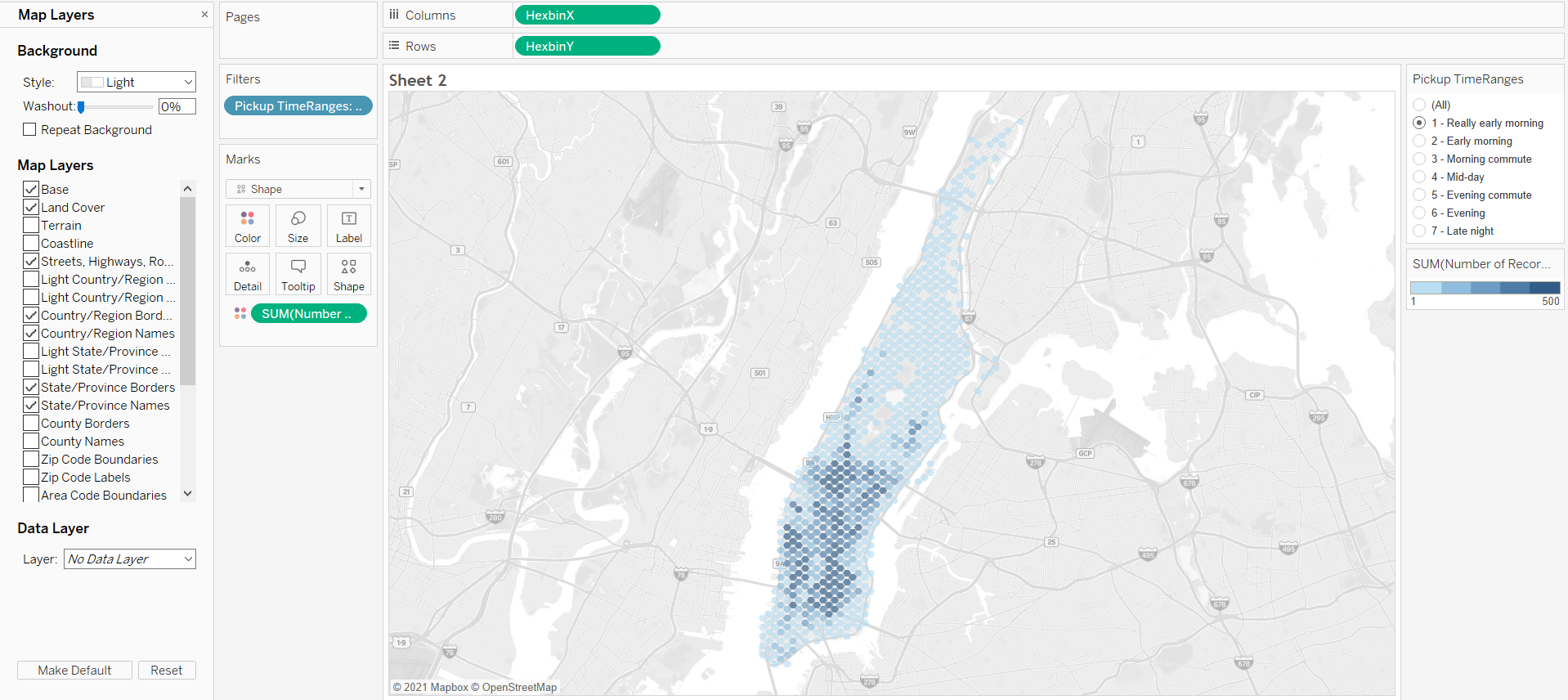
>> Create a hexbin map

<< Goal >>

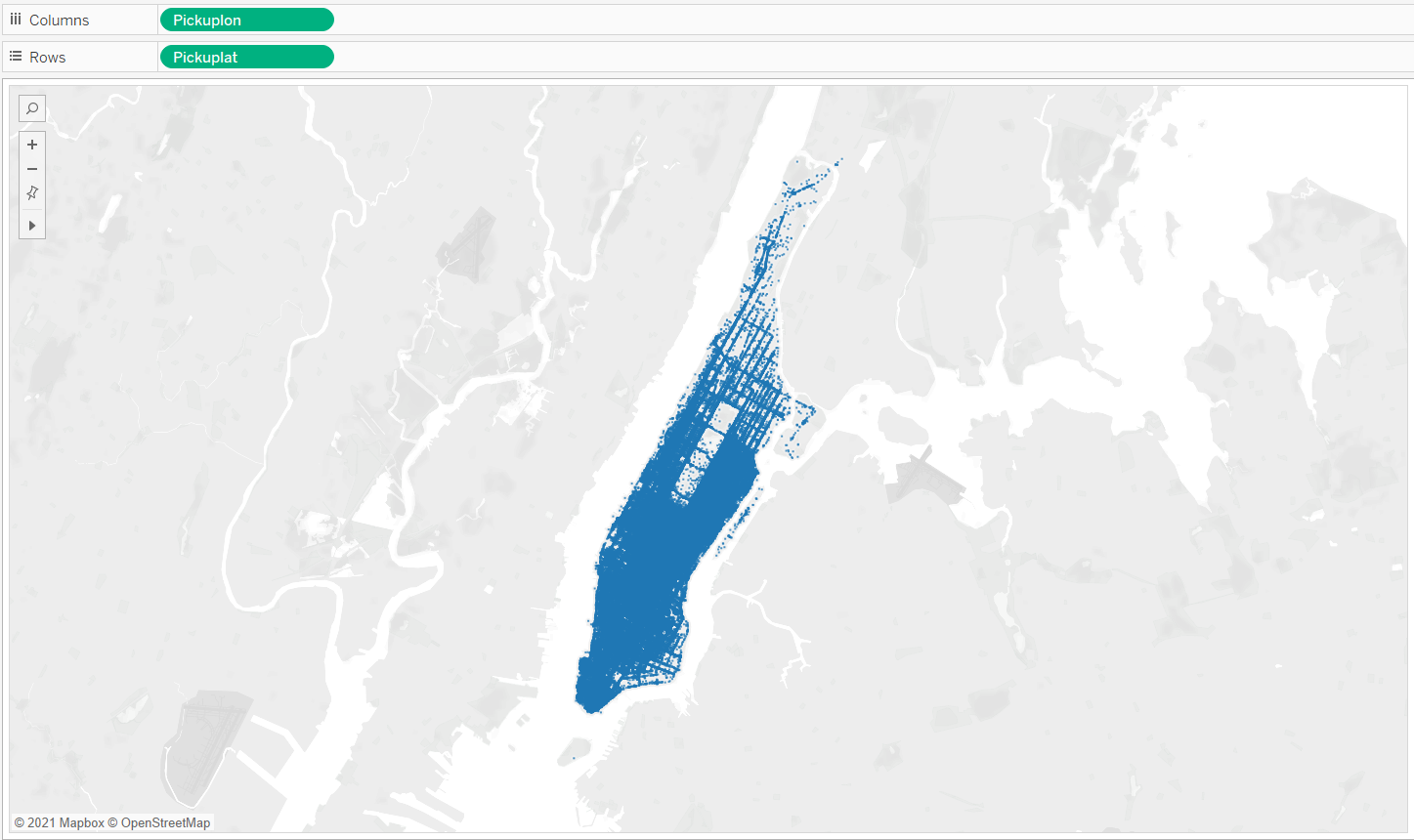
With the data from downtown New York City, we want to see taxi activity by time of day and location.

Create a hexbin map that shows density of taxicab pickups, and filter by the time of day.

<< Process >>

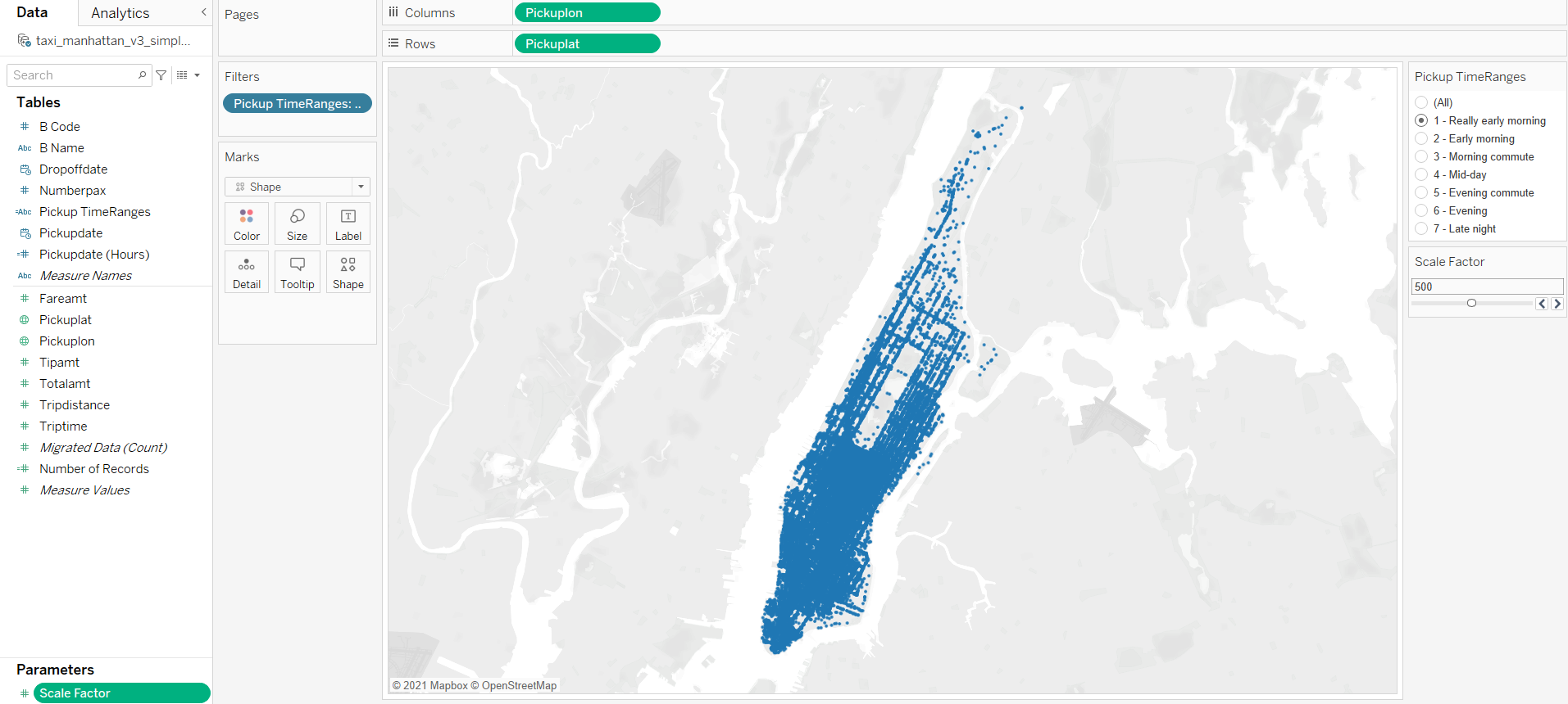
[STEP 1] Build the basic map

• Columns: Pickuplon (set to dimension)
• Rows: Pickuplat (set to dimension)

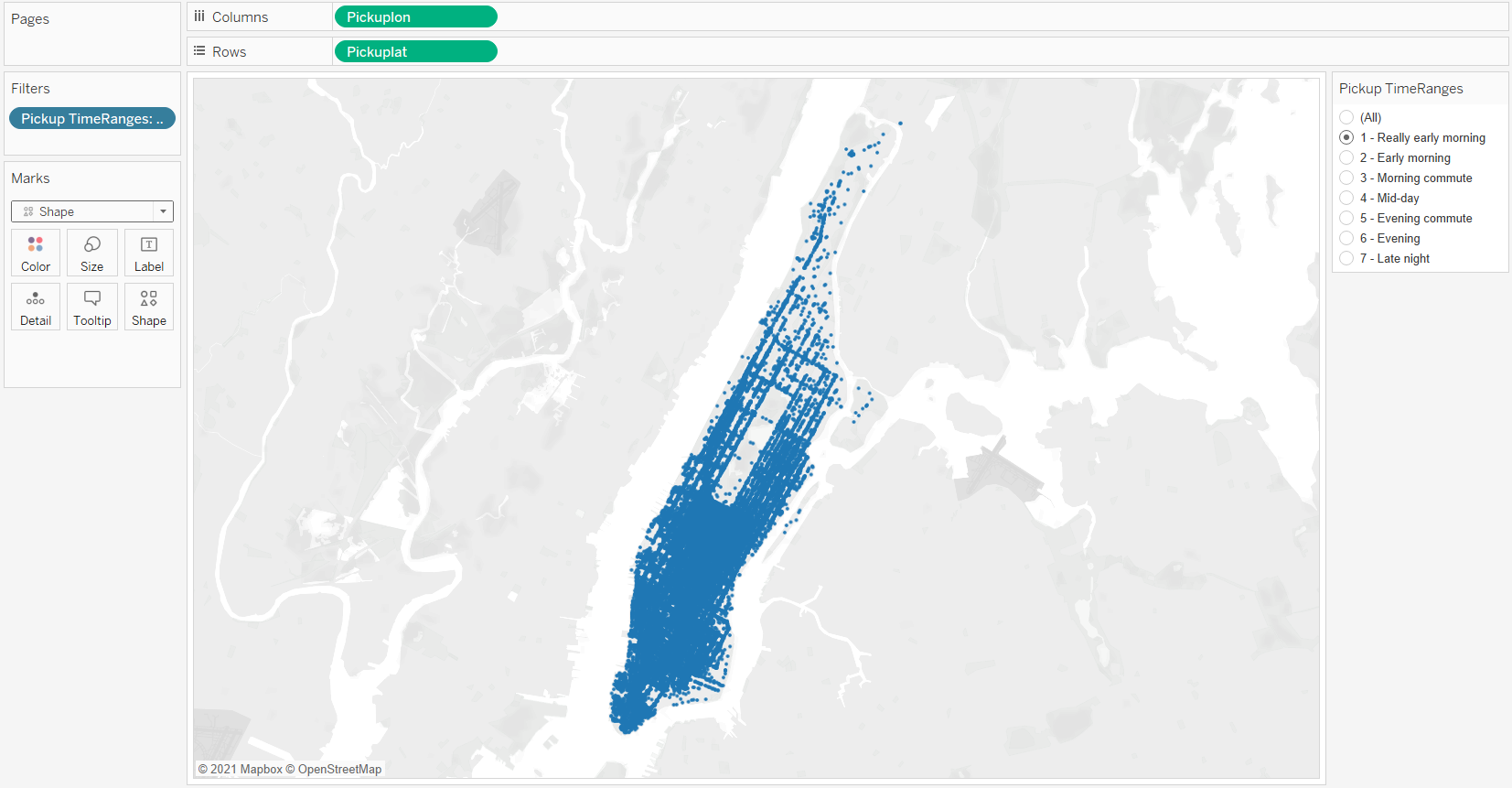
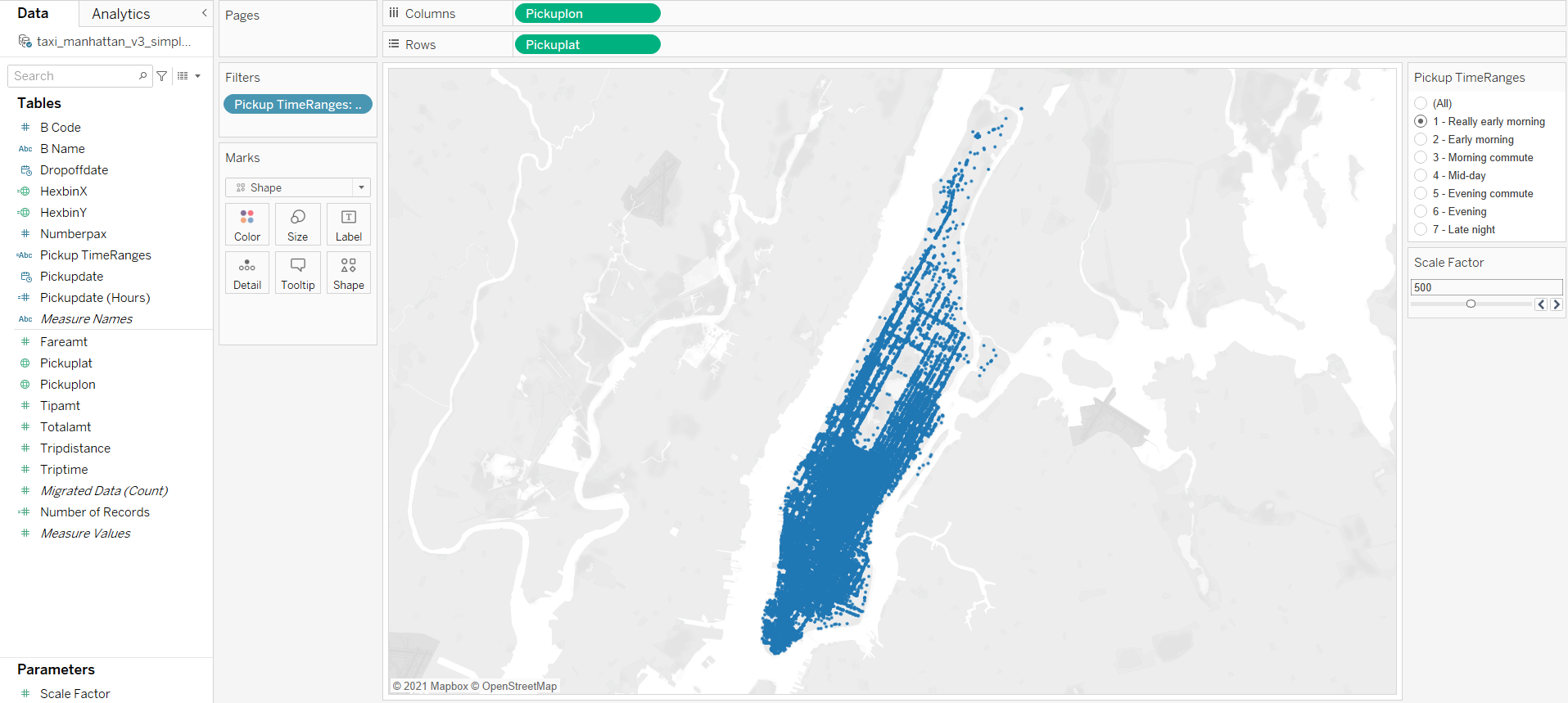
[STEP 2] Filter the view by Pickup TimeRanges, and change the mark type to Shape

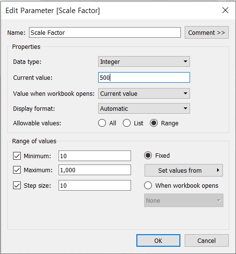
[STEP 3] Create a Scale Factor parameter

[STEP 4] Create HexbinX and HexbinY calculations and set their geographic roles

• Create HexbinX and HexbinY calculations that scale based on the Scale Factor parameter
  • HexbinX: HEXBINX([Pickuplon]*[Scale Factor], [Pickuplat]*[Scale Factor]) / [Scale Factor]
  • HexbinY: HEXBINY([Pickuplon]*[Scale Factor], [Pickuplat]*[Scale Factor]) / [Scale Factor]

• Set the geographic roles of the HexbinX and HexbinY calculations

  • Drag both the HexbinX and HexbinY fields from Measures to Dimensions
  • Set the geographic Role for HexbinX to Longitude, and HexbinY to Latitude
  

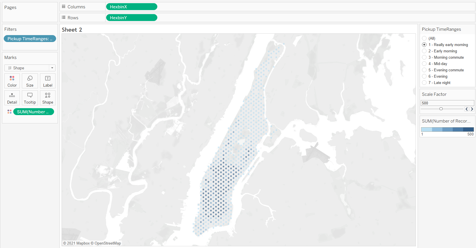
[STEP 5] Update the view with HexbinX and HexbinY, colored by Number of Records

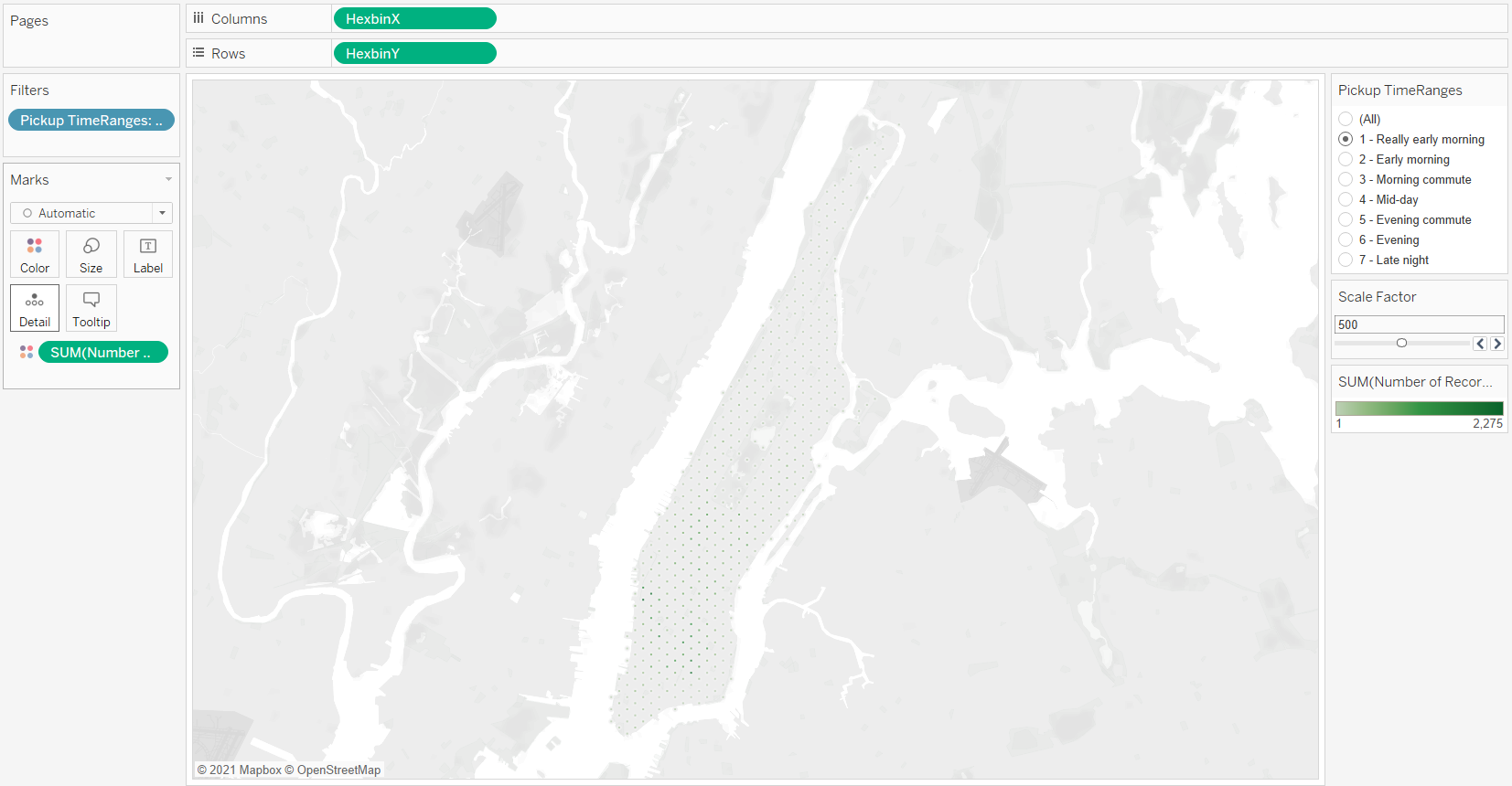
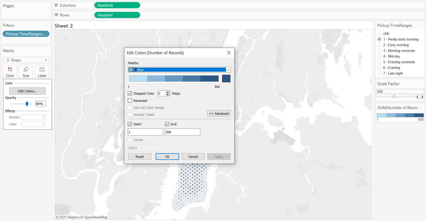
[STEP 6] Edit the color and shape of the marks

• Color:

  • Choose a [Blue] color palette
  • Select [Stepped Color], with 5 steps
  • Click [Advanced] --> adjust the range of the scale: 1 ~ 500
  • transparency: 80%
  

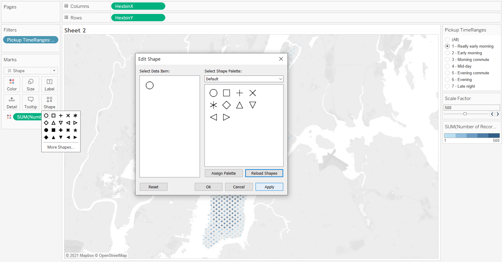
• Shape: Add the hexagon custom shape, and apply the hexagon to the marks in the view

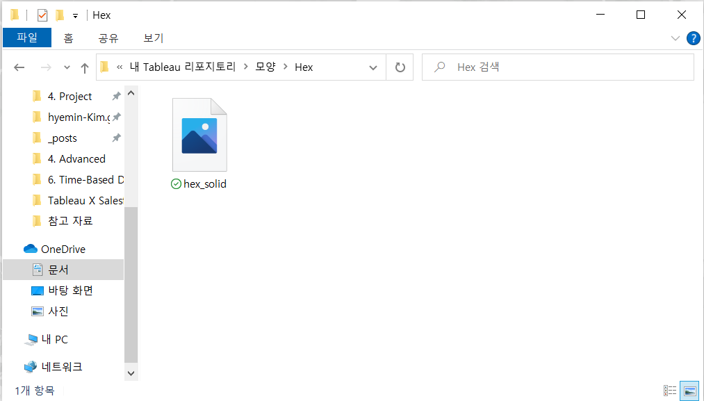
  • Create a new folder called “Hex” in the [My Tableau Repository] --> [Shapes] folder

    - Windows: Documents\My Tableau Repository\Shapes\Hex

    - Mac: Documents/My Tableau Repository/Shapes/Hex

    
    

  • Download or copy the ‘hex_solid.png’ to the Hex folder

    
    

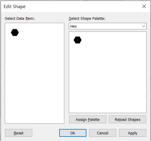
  • [Marks] card --> click [Shape] --> click [More Shapes]

  • Click [Reload Shapes] --> click [Apply]

    
    

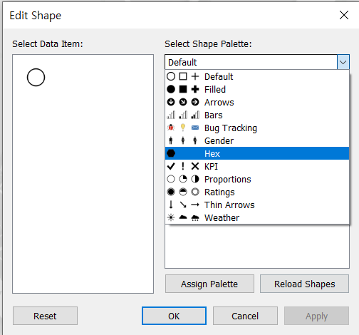
  • [Select Shape Palette] --> select [Hex]

  • Click the solid hexagon image -> click [Apply] -> click [OK]

    

    

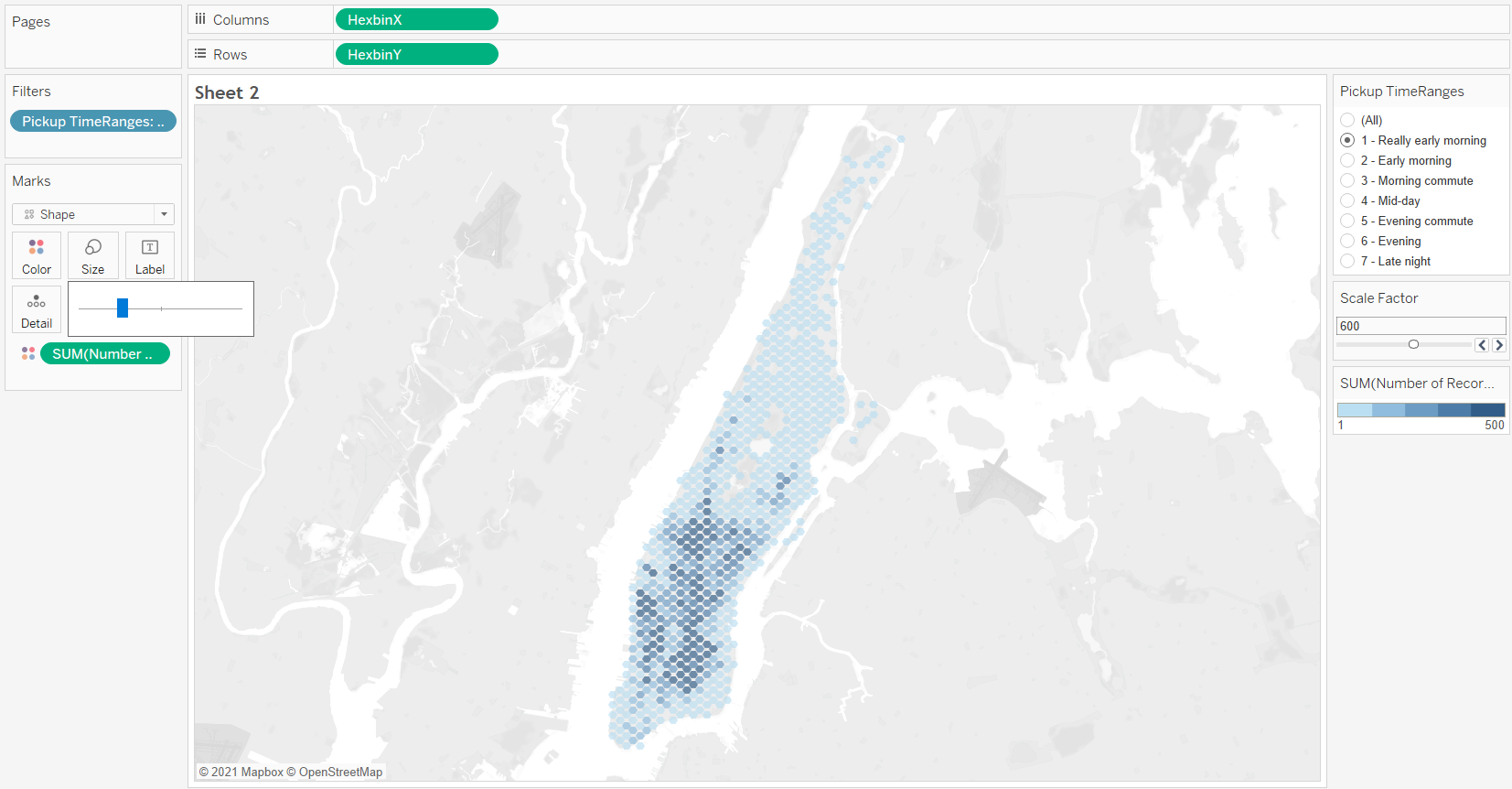
[STEP 7] Adjust the formatting of the view, using the parameter and mark size

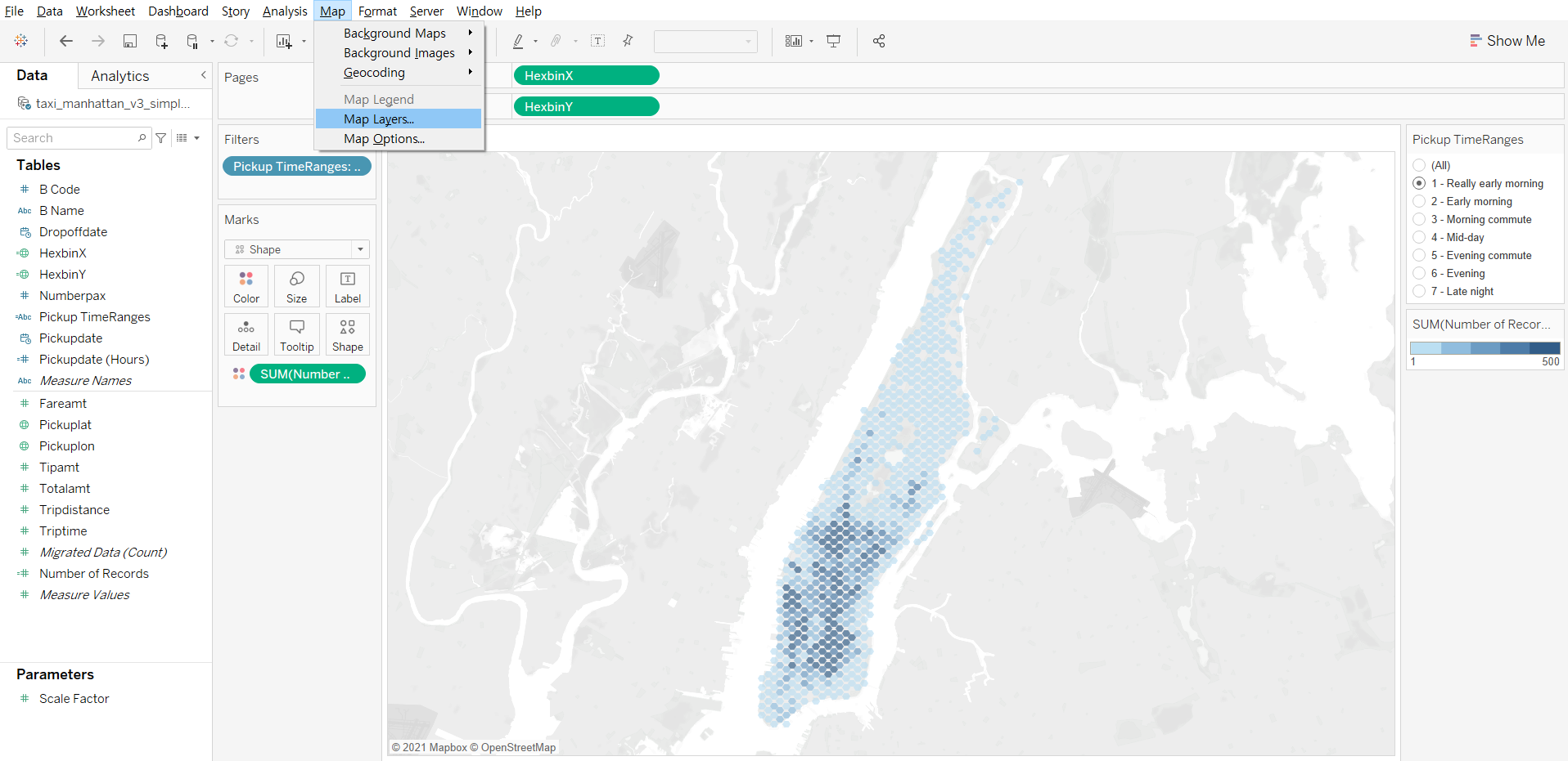
[STEP 8] Update the map layers to show highways

• [Map] --> [Map Layers]

• check [Streets and Highways]

  

2. Map Shapes Using Spatial Files

If geography influences our data questions or business, or location is a vital part of our analysis, we may need to work with spatial files to create maps.

A spatial file contains geographic data that identifies types of natural and man-made features on Earth, and encodes geographic features as geometrical shapes, which we use to visualize and analyze geographic data.

• Three types of geographic features we can use spatial files to map

  • Discrete locations on the ground: wells, mountain peaks, building entrances, or railway stops
  • Geographic features or designations: lakes, farms, park boundaries, neighborhoods, or school districts
  • Linear features: rivers, roads, trails, or highways

• Types of geometrical shapes that Tableau Desktop supports:

  • Points, Circles: for distinct locations on the ground
  • Polygons: for geographic features or designations
  • Lines: for linear features

[Examples]

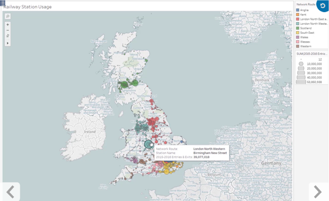
• Locations:

  Show railway stops to explore the frequency of usage at each stop.

  
  

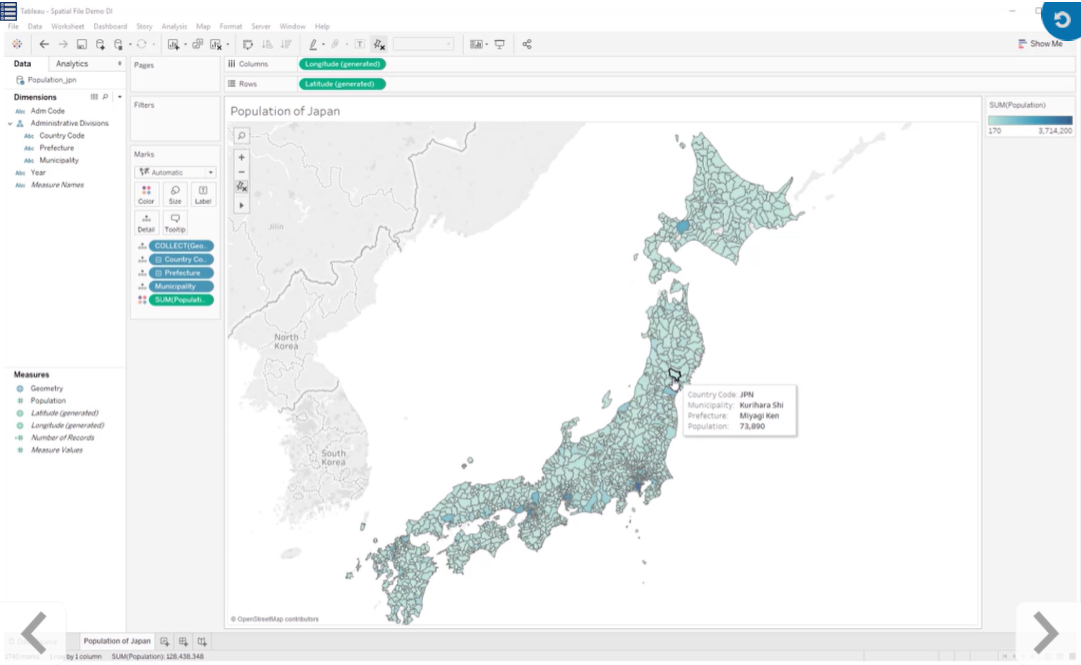
• Areas:

  Show a country’s population broken down by government designations such as prefecture and municipality.

  
  

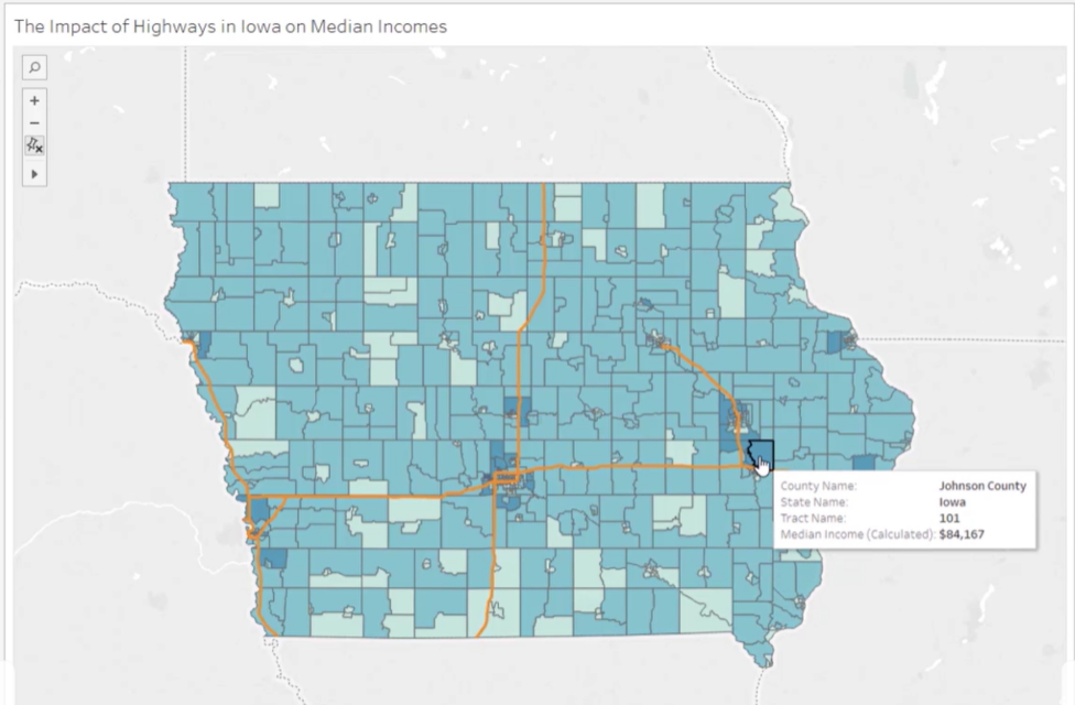
• Linear features:

  Explore the relationship between a highway network and the median income of local residents near it.

  

>> Use spatial files to map data

<< Goal >>

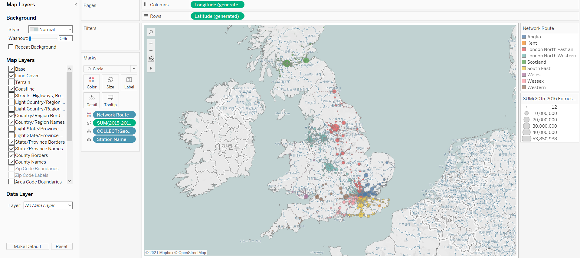
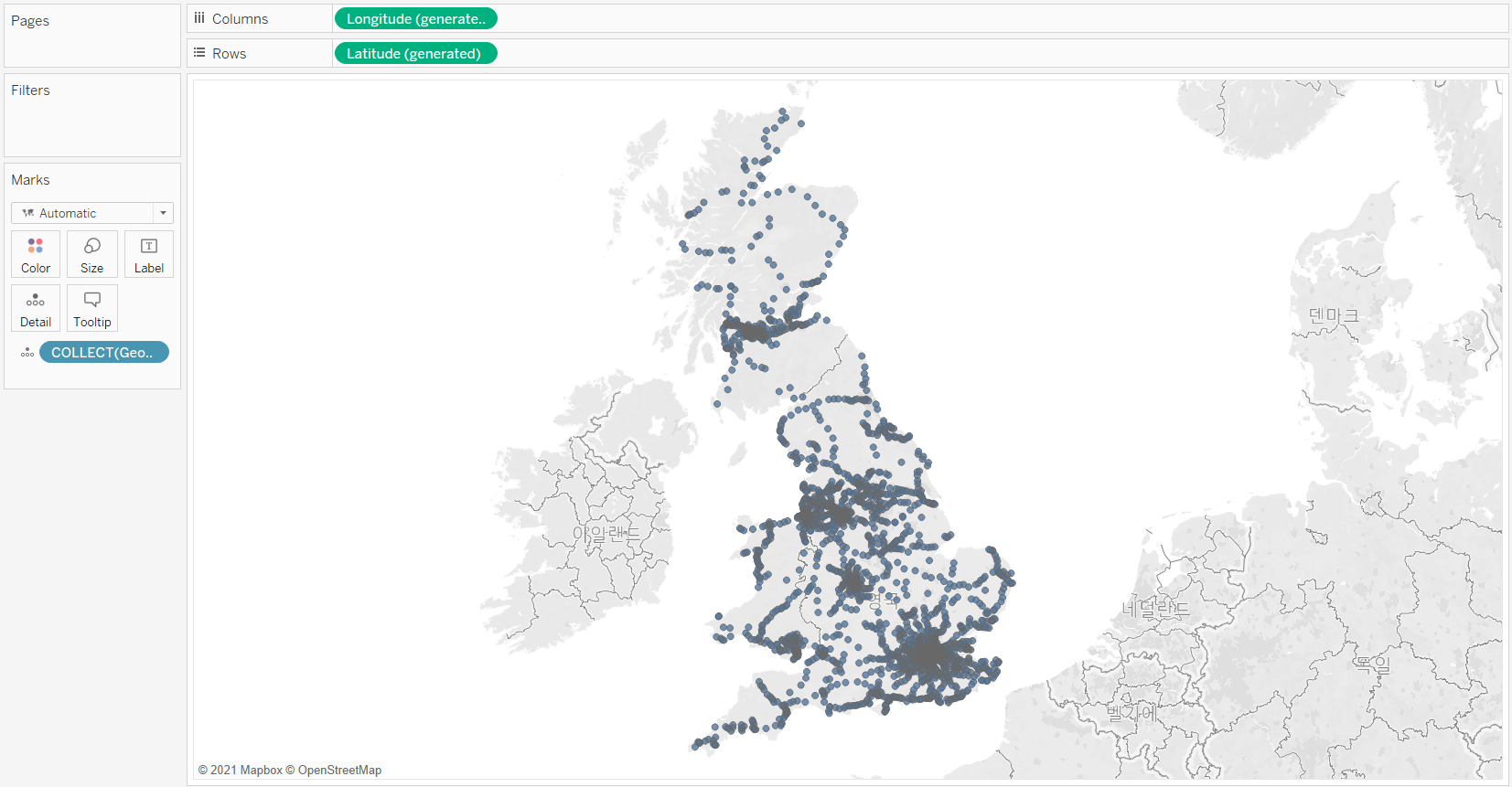
For a study on railway usage in areas of the United Kingdom, we would like to use a spatial file to create a map that shows a network of stations as well as the number of entries and exits, per station, for specific years.

<< Process >>

[STEP 1] Connect to the spatial file

• [Connect] Pane --> [Spatial file]

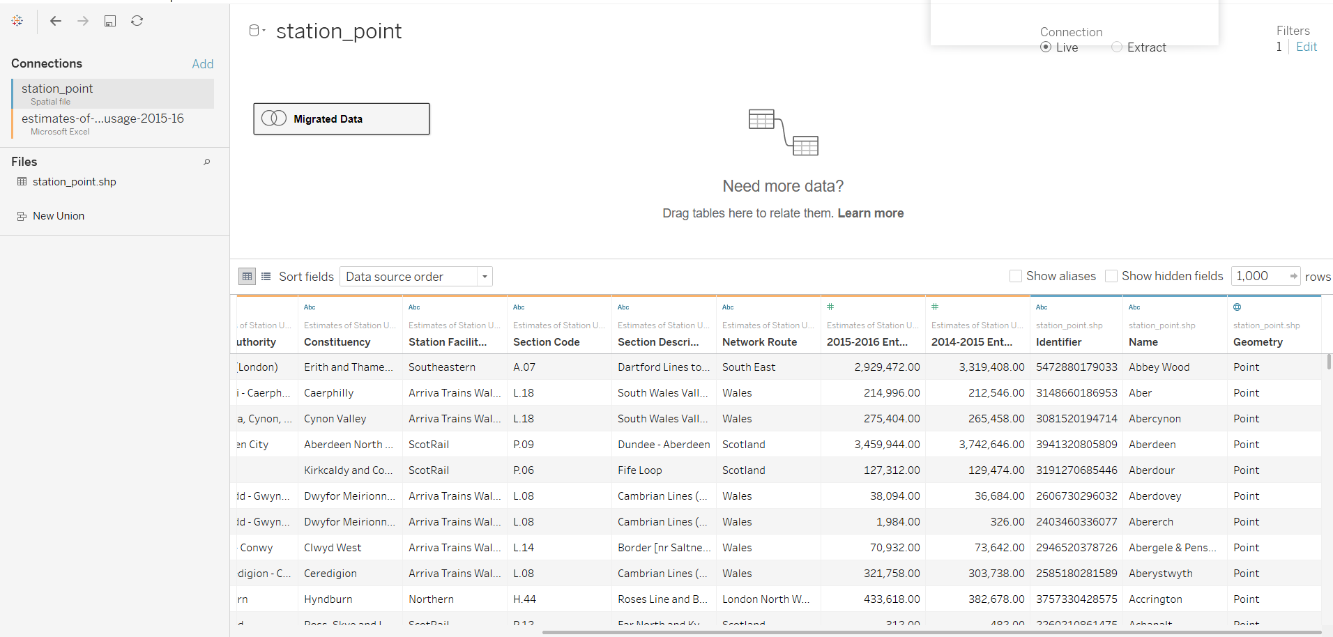
* When connecting to the spatial data, a Geometry field is created to represent the point, polygon, or linear geometries.

[STEP 2] In the worksheet, drag the Geometry field to Detail

* It works in conjunction with latitude and longitude to create the map

* Tableau Desktop aggregates the Geometry measure using the COLLECT aggregation.

​ - By default, the geometry measure is aggregated into a single mark when added to the view

​ - We can add dimensions to disaggregate the data

[STEP 3] Add and Edit the Color, Detail, and Size Marks

• Add Network Route on Color, Station name on Detail, and 2015-2016 Entries & Exits on Size

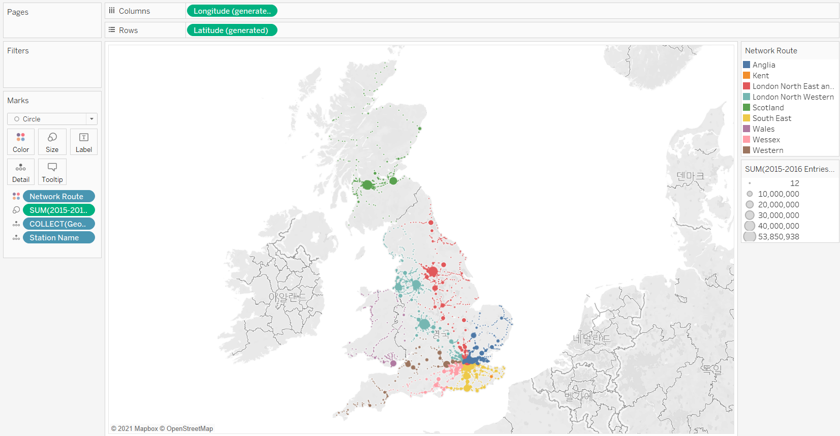
• Increase the mark size, decrease the mark-color opacity, and give marks a gray border.

[STEP 4] Use map layers to edit the background

• Change the background style to [Normal]
• Add the coastline, county borders, and county names